
 GitHub でソースを表示 GitHub でソースを表示 |
はじめに
このノートブックでは、TensorFlow コアの低レベル API を使用して、TensorFlow の高性能科学計算プラットフォームとしての機能を紹介します。TensorFlow Core とその意図するユースケースの詳細については、Core API の概要を参照してください。
このチュートリアルでは、特異値分解(SVD)の手法と、その低階数近似問題への応用について説明します。SVD は、実数または複素数の行列を因数分解するために使用され、画像圧縮などのデータ サイエンスのさまざまなユース ケースがあります。このチュートリアルの画像は、Google Brain の Imagen プロジェクトからのものです。
セットアップ
import matplotlib
from matplotlib.image import imread
from matplotlib import pyplot as plt
import requests
# Preset Matplotlib figure sizes.
matplotlib.rcParams['figure.figsize'] = [16, 9]
import tensorflow as tf
print(tf.__version__)
2024-01-11 18:58:20.567535: E external/local_xla/xla/stream_executor/cuda/cuda_dnn.cc:9261] Unable to register cuDNN factory: Attempting to register factory for plugin cuDNN when one has already been registered
2024-01-11 18:58:20.567578: E external/local_xla/xla/stream_executor/cuda/cuda_fft.cc:607] Unable to register cuFFT factory: Attempting to register factory for plugin cuFFT when one has already been registered
2024-01-11 18:58:20.569139: E external/local_xla/xla/stream_executor/cuda/cuda_blas.cc:1515] Unable to register cuBLAS factory: Attempting to register factory for plugin cuBLAS when one has already been registered
2.15.0
SVD の基礎
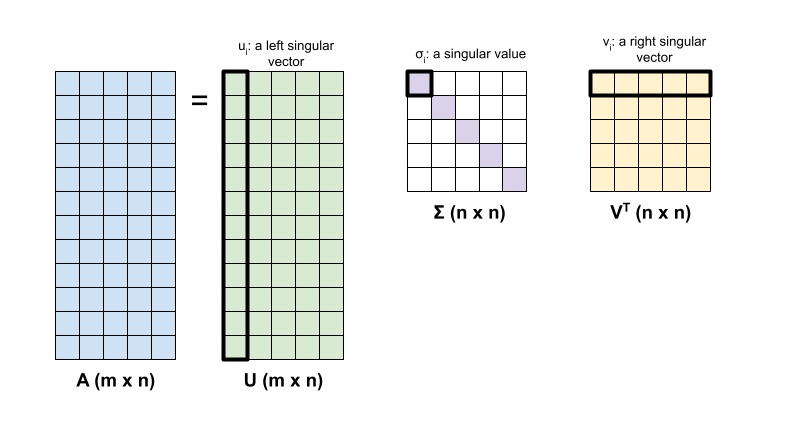
行列の特異値分解 \({\mathrm{A} }\) は、次の因数分解によって決定されます。
\[{\mathrm{A} } = {\mathrm{U} } \Sigma {\mathrm{V} }^T\]
ここでは、それぞれ以下を意味します。
- \(\underset{m \times n}{\mathrm{A} }\): 入力行列、\(m \geq n\)
- \(\underset{m \times n}{\mathrm{U} }\): 直交行列、 \({\mathrm{U} }^T{\mathrm{U} } = {\mathrm{I} }\) 各列で \(u_i\)、\({\mathrm{A} }\) の左特異ベクトルを表す
- \(\underset{n \times n}{\Sigma}\): 各対角要素を持つ対角行列、\(\sigma_i\)、\({\mathrm{A} }\) の特異値を表す
- \(\underset{n \times n}{ {\mathrm{V} }^T}\): 直交行列、\({\mathrm{V} }^T{\mathrm{V} } = {\mathrm{I} }\)、各行 \(v_i\) は、\({\mathrm{A} }\) の右特異ベクトルを表す
\(m < n\) の場合、\({\mathrm{U} }\) と \(\Sigma\) の次元はともに \((m \times m)\) であり、\({\mathrm{V} }^T\) の次元は \((m \times n)\) です。
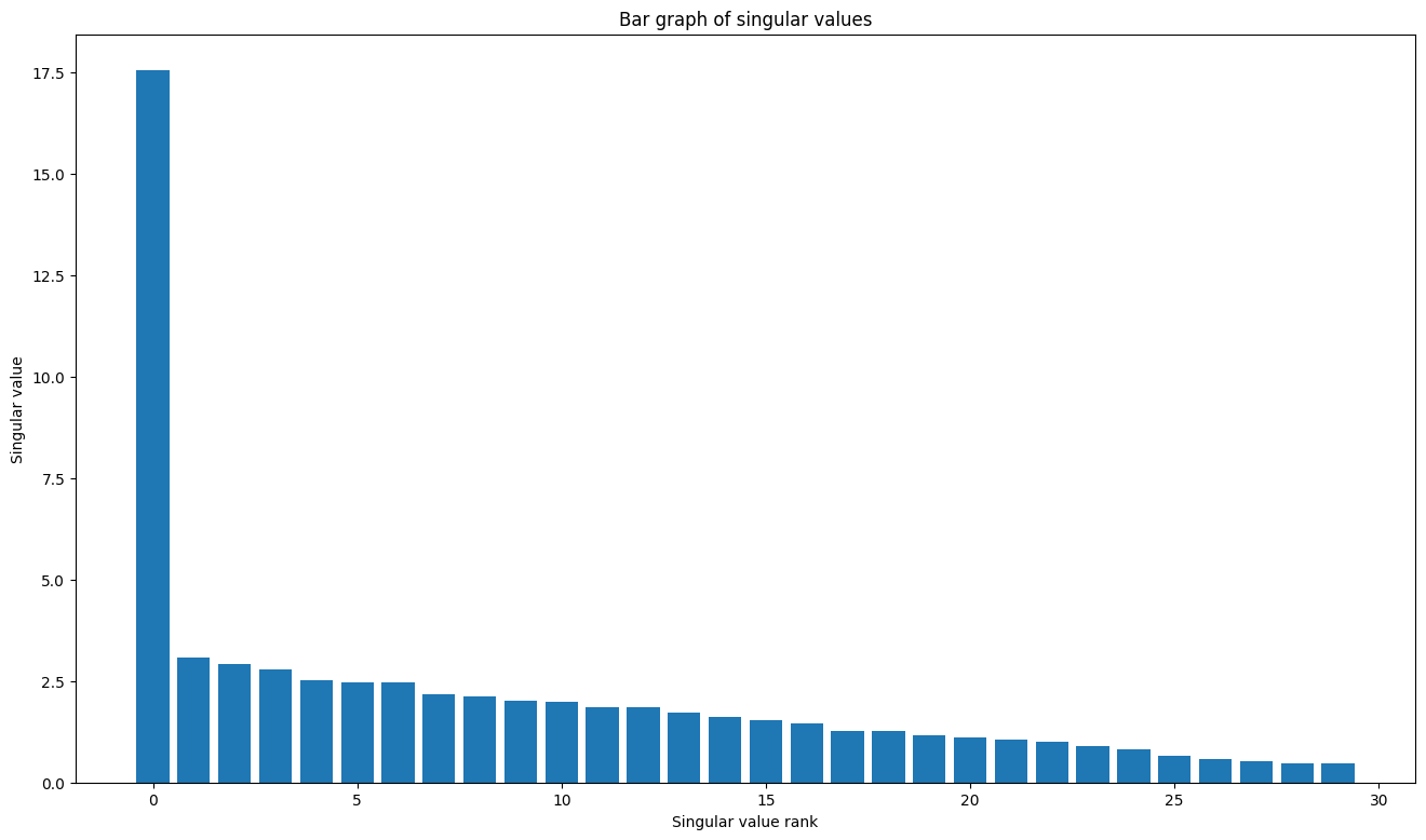
TensorFlow の線形代数パッケージには関数 tf.linalg.svd があり、1 つ以上の行列の特異値分解を計算するために使用できます。まず、単純な行列を定義し、その SVD 因数分解を計算します。
A = tf.random.uniform(shape=[40,30])
# Compute the SVD factorization
s, U, V = tf.linalg.svd(A)
# Define Sigma and V Transpose
S = tf.linalg.diag(s)
V_T = tf.transpose(V)
# Reconstruct the original matrix
A_svd = U@S@V_T
# Visualize
plt.bar(range(len(s)), s);
plt.xlabel("Singular value rank")
plt.ylabel("Singular value")
plt.title("Bar graph of singular values");
tf.einsum 関数を使用すると tf.linalg.svd の出力から行列再構成を直接計算できます。
A_svd = tf.einsum('s,us,vs -> uv',s,U,V)
print('\nReconstructed Matrix, A_svd', A_svd)
Reconstructed Matrix, A_svd tf.Tensor(
[[0.24423978 0.23371103 0.8601791  ... 0.35697114 0.6349882  0.01121274]
 [0.03313616 0.46523762 0.32952744 ... 0.47690722 0.66670346 0.4530385 ]
 [0.21022822 0.5590605  0.3274612  ... 0.13190486 0.25444913 0.19681257]
 ...
 [0.8077496  0.5727718  0.36840475 ... 0.5012198  0.36589172 0.25300917]
 [0.3577813  0.8795756  0.46118328 ... 0.03130534 0.79266065 0.28272972]
 [0.99390686 0.659782   0.25883475 ... 0.42169708 0.35663527 0.03050409]], shape=(40, 30), dtype=float32)
SVD による低階数近似
行列 \({\mathrm{A} }\) の階数は、その列がまたがるベクトル空間の次元によって決まります。SVD は、より低い階数の行列を近似するために使用し、その結果として行列によって表される情報を格納するために必要なデータの次元を削減できます。
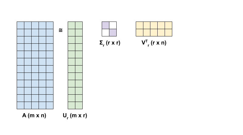
SVD による \({\mathrm{A} }\) の階数 r 近似は、次の式で定義されます。
\[{\mathrm{A_r} } = {\mathrm{U_r} } \Sigma_r {\mathrm{V_r} }^T\]
ここでは、それぞれ以下を意味します。
- \(\underset{m \times r}{\mathrm{U_r} }\): \({\mathrm{U} }\) の最初の \(r\) 列からなる行列
- \(\underset{r \times r}{\Sigma_r}\): \(\Sigma\) の最初の \(r\) 特異値からなる対角行列
- \(\underset{r \times n}{\mathrm{V_r} }^T\): \({\mathrm{V} }^T\) の最初の \(r\) 行からなる行列
まず、与えられた行列の階数 r 近似を計算する関数を記述します。この低階数近似手順は、画像圧縮に使用されます。したがって、各概算の物理データサイズを計算することにも役立ちます。 次に、元の行列 \(\mathrm{A}\) の階数 r 近似 \(\mathrm{A}_r\) と誤差行列 \(|\mathrm{A} - \mathrm{A}_r|\) を視覚化する関数を記述します。
def rank_r_approx(s, U, V, r, verbose=False):
# Compute the matrices necessary for a rank-r approximation
s_r, U_r, V_r = s[..., :r], U[..., :, :r], V[..., :, :r] # ... implies any number of extra batch axes
# Compute the low-rank approximation and its size
A_r = tf.einsum('...s,...us,...vs->...uv',s_r,U_r,V_r)
A_r_size = tf.size(U_r) + tf.size(s_r) + tf.size(V_r)
if verbose:
print(f"Approximation Size: {A_r_size}")
return A_r, A_r_size
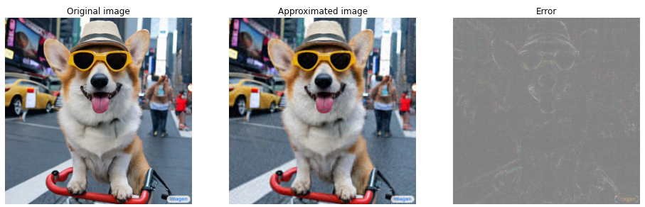
def viz_approx(A, A_r):
# Plot A, A_r, and A - A_r
vmin, vmax = 0, tf.reduce_max(A)
fig, ax = plt.subplots(1,3)
mats = [A, A_r, abs(A - A_r)]
titles = ['Original A', 'Approximated A_r', 'Error |A - A_r|']
for i, (mat, title) in enumerate(zip(mats, titles)):
ax[i].pcolormesh(mat, vmin=vmin, vmax=vmax)
ax[i].set_title(title)
ax[i].axis('off')
print(f"Original Size of A: {tf.size(A)}")
s, U, V = tf.linalg.svd(A)
Original Size of A: 1200
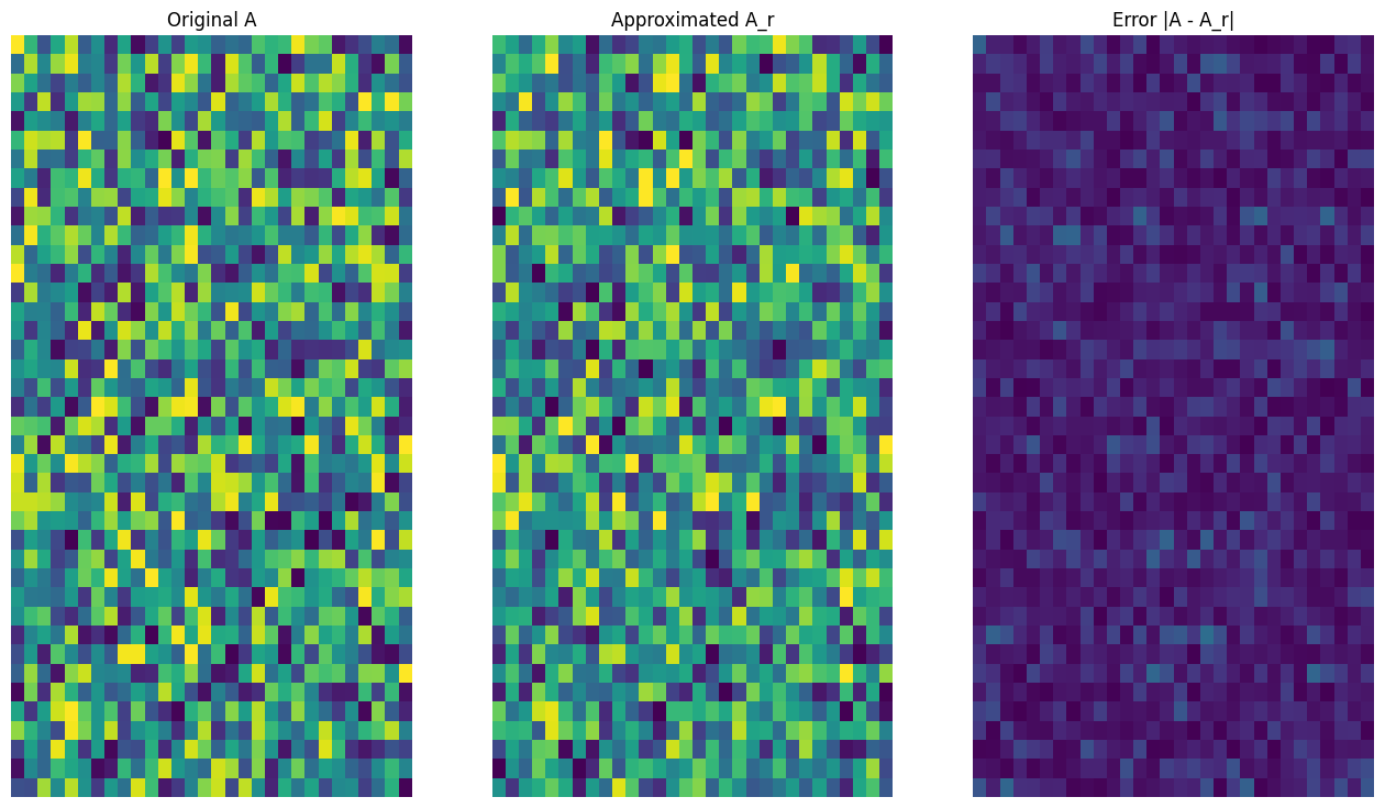
# Rank-15 approximation
A_15, A_15_size = rank_r_approx(s, U, V, 15, verbose = True)
viz_approx(A, A_15)
Approximation Size: 1065
# Rank-3 approximation
A_3, A_3_size = rank_r_approx(s, U, V, 3, verbose = True)
viz_approx(A, A_3)
Approximation Size: 213
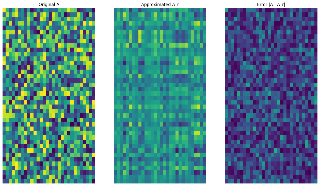
予想どおり、低い階数を使用すると、近似の精度が低下しますが、多くの場合、現実のシナリオでは低階数近似の品質は十分です。また、SVD を使用した低階数近似の主な目的は、データの次元を削減することで、データ自体のディスク領域を削減することではありませんが、入力行列が高次元になると、多く場合、低階数近似によりデータサイズを削減できます。この利点のため、このプロセスは画像圧縮の問題に適用できます。
画像の読み込み
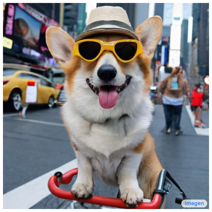
次の画像は、Imagen ホームページで入手できます。Imagen は、Google Research の Brain チームによって開発されたテキストから画像を生成する拡散モデルです。AI は、「タイムズスクエアで自転車に乗っているコーギー犬の写真。この犬はサングラスをかけてビーチハットをかぶっている。」というプロンプトに基づいて、この画像を作成しました。なんてクールなのでしょう! また、以下の URL を任意の .jpg リンクに変更して、選択したカスタム画像を読み込むこともできます。
画像を読み込んで視覚化することから始めます。 JPEG ファイルを読み取った後、Matplotlib は行列 \({\mathrm{I} }\) を \((m \times n \times 3)\) の形状で出力します。これは、それぞれ赤、緑、青の 3 つのカラー チャネルを持つ 2 次元画像を表します。
img_link = "https://imagen.research.google/main_gallery_images/a-photo-of-a-corgi-dog-riding-a-bike-in-times-square.jpg"
img_path = requests.get(img_link, stream=True).raw
I = imread(img_path, 0)
print("Input Image Shape:", I.shape)
Input Image Shape: (1024, 1024, 3)
def show_img(I):
  # Display the image in matplotlib
  img = plt.imshow(I)
  plt.axis('off')
  return
show_img(I)
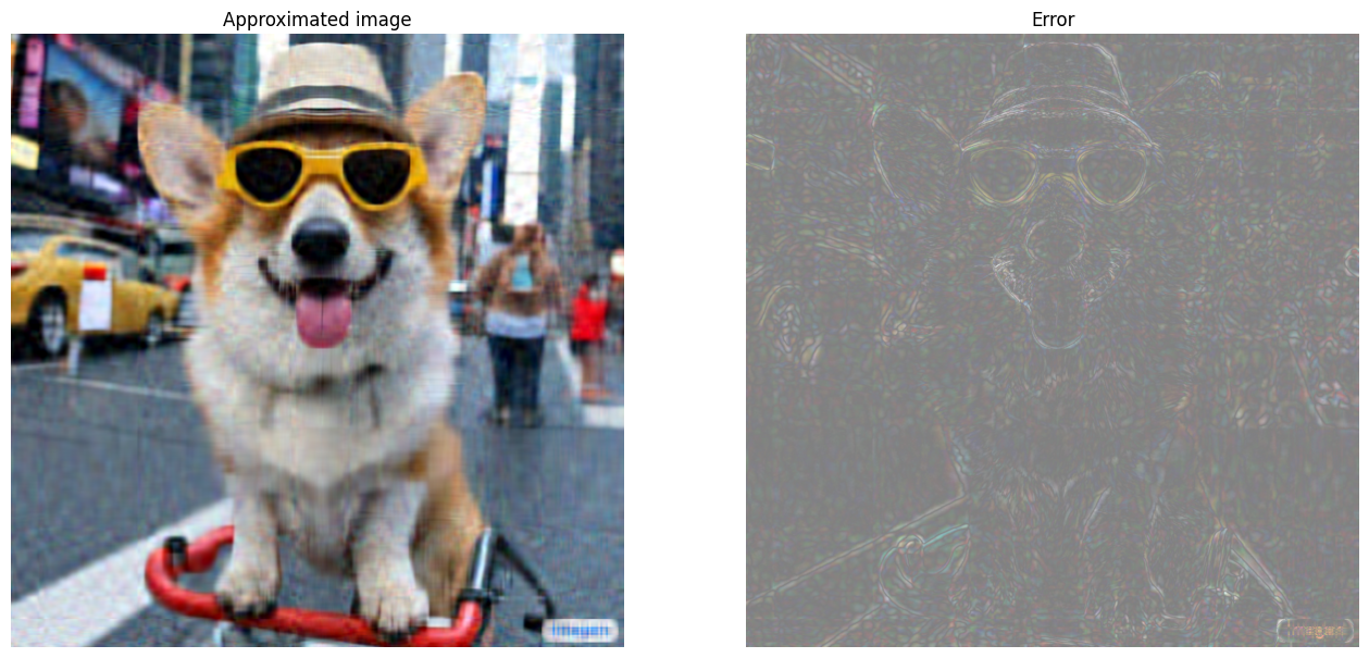
画像圧縮アルゴリズム
次に、SVD を使用して、サンプル画像の低階数近似を計算します。画像の形状は \((1024 \times 1024 \times 3)\) であり、SVD 理論は 2 次元行列にのみ適用されます。これは、サンプル画像を、3 つのカラー チャネルのそれぞれに対応する 3 つの等しいサイズの行列にバッチ処理する必要があることを意味します。そのためには、行列を \((3 \times 1024 \times 1024)\) の形状になるように転置します。近似誤差を明確に視覚化するために、画像の RGB 値を \([0,255]\) から \([0,1]\) に再スケーリングします。概算値を視覚化する前に、この間隔内に収まるようにクリップすることを忘れないでください。これには tf.clip_by_value 関数が役立ちます。
def compress_image(I, r, verbose=False):
  # Compress an image with the SVD given a rank
  I_size = tf.size(I)
  print(f"Original size of image: {I_size}")
  # Compute SVD of image
  I = tf.convert_to_tensor(I)/255
  I_batched = tf.transpose(I, [2, 0, 1]) # einops.rearrange(I, 'h w c -> c h w')
  s, U, V = tf.linalg.svd(I_batched)
  # Compute low-rank approximation of image across each RGB channel
  I_r, I_r_size = rank_r_approx(s, U, V, r)
  I_r = tf.transpose(I_r, [1, 2, 0]) # einops.rearrange(I_r, 'c h w -> h w c')
  I_r_prop = (I_r_size / I_size)
  if verbose:
    # Display compressed image and attributes
    print(f"Number of singular values used in compression: {r}")
    print(f"Compressed image size: {I_r_size}")
    print(f"Proportion of original size: {I_r_prop:.3f}")
    ax_1 = plt.subplot(1,2,1)
    show_img(tf.clip_by_value(I_r,0.,1.))
    ax_1.set_title("Approximated image")
    ax_2 = plt.subplot(1,2,2)
    show_img(tf.clip_by_value(0.5+abs(I-I_r),0.,1.))
    ax_2.set_title("Error")
  return I_r, I_r_prop
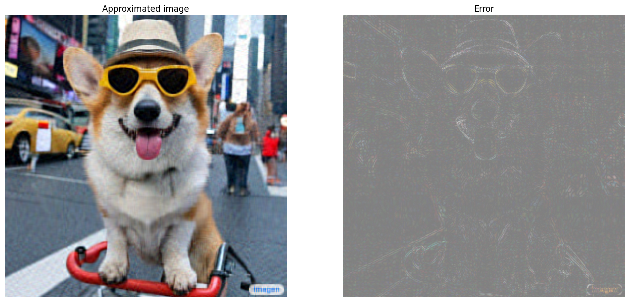
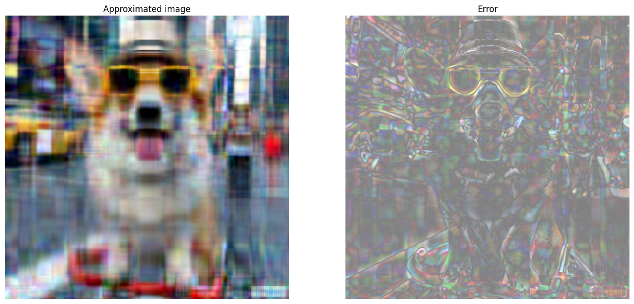
次に、次の階数の階数 r 近似を計算します: 100、50、10
I_100, I_100_prop = compress_image(I, 100, verbose=True)
Original size of image: 3145728
Number of singular values used in compression: 100
Compressed image size: 614700
Proportion of original size: 0.195
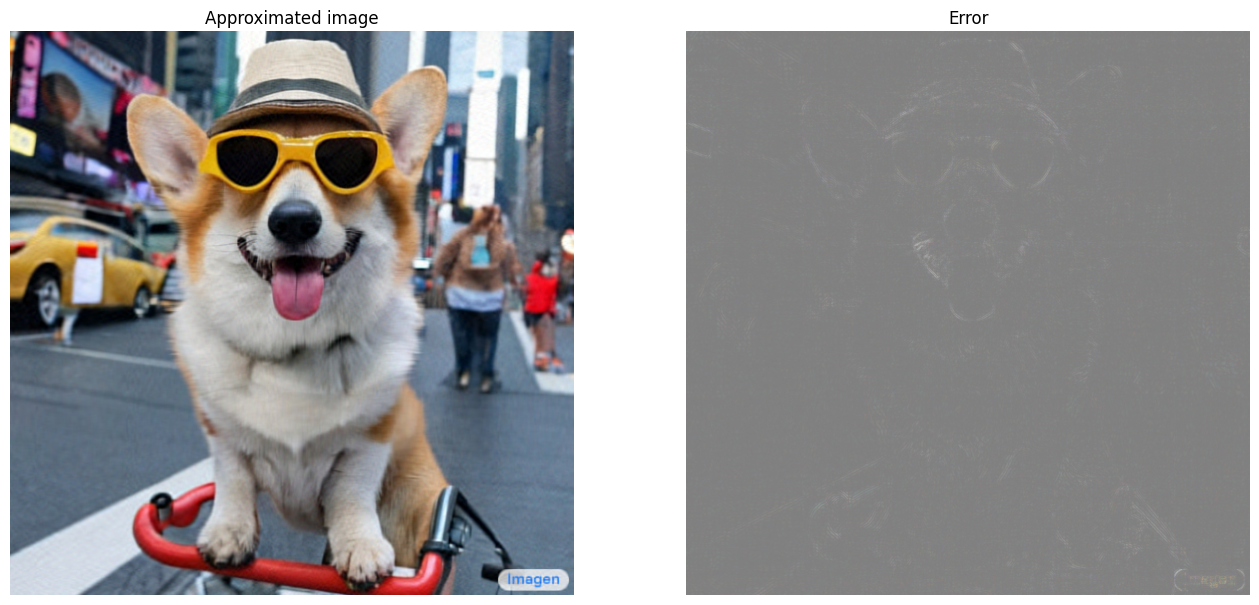
I_50, I_50_prop = compress_image(I, 50, verbose=True)
Original size of image: 3145728
Number of singular values used in compression: 50
Compressed image size: 307350
Proportion of original size: 0.098
I_10, I_10_prop = compress_image(I, 10, verbose=True)
Original size of image: 3145728
Number of singular values used in compression: 10
Compressed image size: 61470
Proportion of original size: 0.020
近似の評価
様々な興味深い方法で有効性を測定し、行列近似をより詳細に制御できます。
圧縮係数と階数
上記の各近似値について、階数によってデータサイズがどのように変化するかを観察します。
plt.figure(figsize=(11,6))
plt.plot([100, 50, 10], [I_100_prop, I_50_prop, I_10_prop])
plt.xlabel("Rank")
plt.ylabel("Proportion of original image size")
plt.title("Compression factor vs rank");
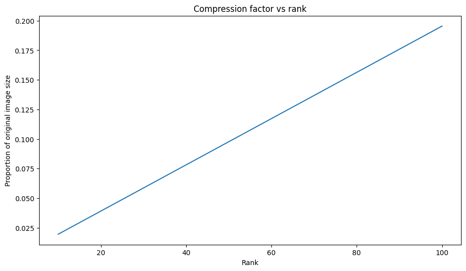
このプロットに基づくと、近似画像の圧縮係数とその階数の間に線形関係があります。これをさらに詳しく調べるには、近似行列のデータサイズ \({\mathrm{A} }_r\) が、その計算に必要な要素の総数として定義されていることを思い出してください。次の式を使用して、圧縮係数と階数の関係を見つけることができます。
\[x = (m \times r) + r + (r \times n) = r \times (m + n + 1)\]
\[c = \large \frac{x}{y} = \frac{r \times (m + n + 1)}{m \times n}\]
ここでは、それぞれ以下を意味します。
- \(x\): \({\mathrm{A_r} }\) のサイズ
- \(y\): \({\mathrm{A} }\) のサイズ
- \(c = \frac{x}{y}\): 圧縮係数
- \(r\): 近似の階数
- \(m\) と \(n\): \({\mathrm{A} }\) の行と列の次元
画像を希望する係数 \(c\) に圧縮するために必要な階数 \(r\) を求めるには、上記の式を並べ替えて \(r\) を求めます。
\[r = ⌊{\large\frac{c \times m \times n}{m + n + 1} }⌋\]
各 RGB 近似は互いに影響しないため、この式はカラーチャネルの次元とは無関係であることに注意してください。次に、希望する圧縮係数を指定して入力画像を圧縮する関数を作成します。
def compress_image_with_factor(I, compression_factor, verbose=False):
  # Returns a compressed image based on a desired compression factor
  m,n,o = I.shape
  r = int((compression_factor * m * n)/(m + n + 1))
  I_r, I_r_prop = compress_image(I, r, verbose=verbose)
  return I_r
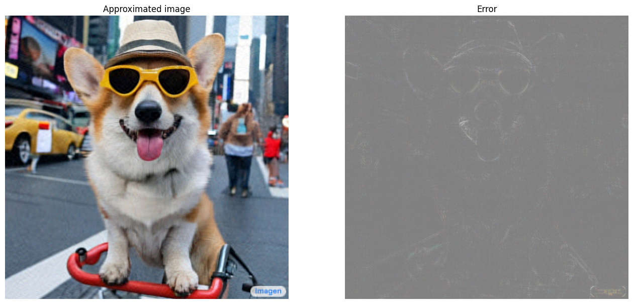
画像を元のサイズの 15% に圧縮します。
compression_factor = 0.15
I_r_img = compress_image_with_factor(I, compression_factor, verbose=True)
Original size of image: 3145728
Number of singular values used in compression: 76
Compressed image size: 467172
Proportion of original size: 0.149
特異値の累積和
特異値の累積和は、階数 r 近似によって取得されるエネルギー量の有用な指標になる場合があります。サンプル画像内の特異値の RGB 平均累積比率を可視化します。これには tf.cumsum 関数が役立ちます。
def viz_energy(I):
  # Visualize the energy captured based on rank
  # Computing SVD
  I = tf.convert_to_tensor(I)/255
  I_batched = tf.transpose(I, [2, 0, 1])
  s, U, V = tf.linalg.svd(I_batched)
  # Plotting average proportion across RGB channels
  props_rgb = tf.map_fn(lambda x: tf.cumsum(x)/tf.reduce_sum(x), s)
  props_rgb_mean = tf.reduce_mean(props_rgb, axis=0)
  plt.figure(figsize=(11,6))
  plt.plot(range(len(I)), props_rgb_mean, color='k')
  plt.xlabel("Rank / singular value number")
  plt.ylabel("Cumulative proportion of singular values")
  plt.title("RGB-averaged proportion of energy captured by the first 'r' singular values")
viz_energy(I)
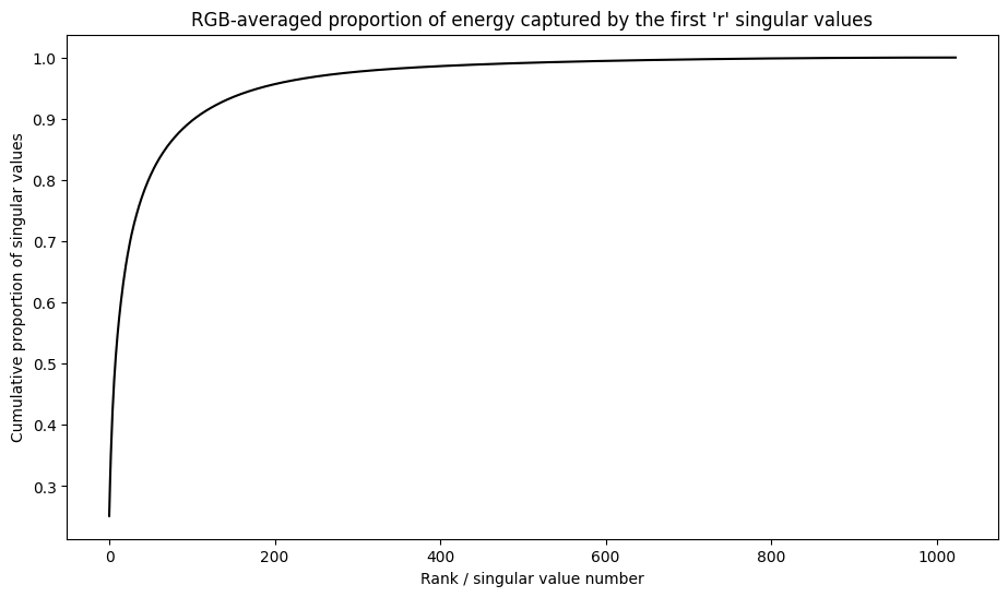
この画像のエネルギーの 90% 以上が、最初の 100 個の特異値にキャプチャされているようです。次に、希望するエネルギー保持率を指定して、入力画像を圧縮する関数を作成します。
def compress_image_with_energy(I, energy_factor, verbose=False):
  # Returns a compressed image based on a desired energy factor
  # Computing SVD
  I_rescaled = tf.convert_to_tensor(I)/255
  I_batched = tf.transpose(I_rescaled, [2, 0, 1])
  s, U, V = tf.linalg.svd(I_batched)
  # Extracting singular values
  props_rgb = tf.map_fn(lambda x: tf.cumsum(x)/tf.reduce_sum(x), s)
  props_rgb_mean = tf.reduce_mean(props_rgb, axis=0)
  # Find closest r that corresponds to the energy factor
  r = tf.argmin(tf.abs(props_rgb_mean - energy_factor)) + 1
  actual_ef = props_rgb_mean[r]
  I_r, I_r_prop = compress_image(I, r, verbose=verbose)
  print(f"Proportion of energy captured by the first {r} singular values: {actual_ef:.3f}")
  return I_r
画像を圧縮して、そのエネルギーの 75% を保持します。
energy_factor = 0.75
I_r_img = compress_image_with_energy(I, energy_factor, verbose=True)
Original size of image: 3145728
Number of singular values used in compression: 35
Compressed image size: 215145
Proportion of original size: 0.068
Proportion of energy captured by the first 35 singular values: 0.753
エラーと特異値
近似誤差と特異値の間にも興味深い関係があります。近似のフロベニウスノルムの 2 乗は、除外された特異値の 2 乗の和に等しいことがわかります。
\[{||A - A_r||}^2 = \sum_{i=r+1}^{R}σ_i^2\]
このチュートリアルの最初にある行列例の階数 10 近似を使用して、この関係をテストしてください。
s, U, V = tf.linalg.svd(A)
A_10, A_10_size = rank_r_approx(s, U, V, 10)
squared_norm = tf.norm(A - A_10)**2
s_squared_sum = tf.reduce_sum(s[10:]**2)
print(f"Squared Frobenius norm: {squared_norm:.3f}")
print(f"Sum of squared singular values left out: {s_squared_sum:.3f}")
Squared Frobenius norm: 31.750
Sum of squared singular values left out: 31.750
まとめ
このノートブックでは、TensorFlow を使用して特異値分解を実装し、それを適用して画像圧縮アルゴリズムを作成するプロセスを紹介しました。以下に役立つヒントをいくつか紹介します。
- TensorFlow Core API は、高性能科学計算のさまざまなユースケースに利用できます。
- TensorFlow の線形代数機能の詳細については、linalg モジュールのドキュメントを参照してください。
- SVD は、レコメンデーションシステムの構築にも適用できます。
TensorFlow Core API のその他の使用例については、チュートリアルを参照してください。データの読み込みと準備についてさらに学習するには、画像データの読み込みまたは CSV データの読み込みに関するチュートリアルを参照してください。