
| |
|
 GitHub でソースを表示 GitHub でソースを表示 |
このノートブックでは、映画レビューのテキストを使用して、それが肯定的であるか否定的であるかに分類します。これは二項分類の例で、機械学習問題では重要な分類法として広く適用されます。
Internet Movie Database より、50,000 件の映画レビューテキストが含まれる IMDB データセットを使用します。これは、トレーニング用の 25,000 件のレビューとテスト用の 25,000 件のレビューに分割されます。トレーニングセットとテストセットは均衡が保たれており、肯定的評価と否定的評価が同じ割合で含まれます。
このノートブックでは、TensorFlow でモデルを構築してトレーニングするための tf.keras という高レベル API と、転移学習用のライブラリ兼プラットフォームである TensorFlow Hub を使用します。tf.keras を使用した、より高度なテキスト分類チュートリアルについては、MLCC Text Classification Guide をご覧ください。
その他のモデル
テキスト埋め込みの生成に使用できる、より表現豊かなモデルや効率性の高いモデルをこちらでご覧ください。
MNIST モデルをビルドする
import numpy as np

import tensorflow as tf
import tensorflow_hub as hub
import tensorflow_datasets as tfds

import matplotlib.pyplot as plt

print("Version: ", tf.__version__)
print("Eager mode: ", tf.executing_eagerly())
print("Hub version: ", hub.__version__)
print("GPU is", "available" if tf.config.list_physical_devices('GPU') else "NOT AVAILABLE")
2024-01-11 19:52:40.814991: E external/local_xla/xla/stream_executor/cuda/cuda_dnn.cc:9261] Unable to register cuDNN factory: Attempting to register factory for plugin cuDNN when one has already been registered
2024-01-11 19:52:40.815032: E external/local_xla/xla/stream_executor/cuda/cuda_fft.cc:607] Unable to register cuFFT factory: Attempting to register factory for plugin cuFFT when one has already been registered
2024-01-11 19:52:40.816571: E external/local_xla/xla/stream_executor/cuda/cuda_blas.cc:1515] Unable to register cuBLAS factory: Attempting to register factory for plugin cuBLAS when one has already been registered
Version:  2.15.0
Eager mode:  True
Hub version:  0.15.0
GPU is available
IMDB データセットをダウンロードする
IMDB データセットは、TensorFlow データセットで提供されています。次のコードを使って、IMDB データセットをマシン(または Colab ランタイム)にダウンロードしてください。
train_data, test_data = tfds.load(name="imdb_reviews", split=["train", "test"],
                                  batch_size=-1, as_supervised=True)

train_examples, train_labels = tfds.as_numpy(train_data)
test_examples, test_labels = tfds.as_numpy(test_data)
データの観察
データの形式を確認してみましょう。各サンプルは、映画レビューを表す文章と対応するラベルです。文章はまったく事前処理されていません。ラベルは 0 または 1 の整数値で、0 は否定的なレビューで 1 は肯定的なレビューを示します。
print("Training entries: {}, test entries: {}".format(len(train_examples), len(test_examples)))
Training entries: 25000, test entries: 25000
最初の 10 個のサンプルを出力しましょう。
train_examples[:10]
array([b"This was an absolutely terrible movie. Don't be lured in by Christopher Walken or Michael Ironside. Both are great actors, but this must simply be their worst role in history. Even their great acting could not redeem this movie's ridiculous storyline. This movie is an early nineties US propaganda piece. The most pathetic scenes were those when the Columbian rebels were making their cases for revolutions. Maria Conchita Alonso appeared phony, and her pseudo-love affair with Walken was nothing but a pathetic emotional plug in a movie that was devoid of any real meaning. I am disappointed that there are movies like this, ruining actor's like Christopher Walken's good name. I could barely sit through it.",
       b'I have been known to fall asleep during films, but this is usually due to a combination of things including, really tired, being warm and comfortable on the sette and having just eaten a lot. However on this occasion I fell asleep because the film was rubbish. The plot development was constant. Constantly slow and boring. Things seemed to happen, but with no explanation of what was causing them or why. I admit, I may have missed part of the film, but i watched the majority of it and everything just seemed to happen of its own accord without any real concern for anything else. I cant recommend this film at all.',
       b'Mann photographs the Alberta Rocky Mountains in a superb fashion, and Jimmy Stewart and Walter Brennan give enjoyable performances as they always seem to do. <br /><br />But come on Hollywood - a Mountie telling the people of Dawson City, Yukon to elect themselves a marshal (yes a marshal!) and to enforce the law themselves, then gunfighters battling it out on the streets for control of the town? <br /><br />Nothing even remotely resembling that happened on the Canadian side of the border during the Klondike gold rush. Mr. Mann and company appear to have mistaken Dawson City for Deadwood, the Canadian North for the American Wild West.<br /><br />Canadian viewers be prepared for a Reefer Madness type of enjoyable howl with this ludicrous plot, or, to shake your head in disgust.',
       b'This is the kind of film for a snowy Sunday afternoon when the rest of the world can go ahead with its own business as you descend into a big arm-chair and mellow for a couple of hours. Wonderful performances from Cher and Nicolas Cage (as always) gently row the plot along. There are no rapids to cross, no dangerous waters, just a warm and witty paddle through New York life at its best. A family film in every sense and one that deserves the praise it received.',
       b'As others have mentioned, all the women that go nude in this film are mostly absolutely gorgeous. The plot very ably shows the hypocrisy of the female libido. When men are around they want to be pursued, but when no "men" are around, they become the pursuers of a 14 year old boy. And the boy becomes a man really fast (we should all be so lucky at this age!). He then gets up the courage to pursue his true love.',
       b"This is a film which should be seen by anybody interested in, effected by, or suffering from an eating disorder. It is an amazingly accurate and sensitive portrayal of bulimia in a teenage girl, its causes and its symptoms. The girl is played by one of the most brilliant young actresses working in cinema today, Alison Lohman, who was later so spectacular in 'Where the Truth Lies'. I would recommend that this film be shown in all schools, as you will never see a better on this subject. Alison Lohman is absolutely outstanding, and one marvels at her ability to convey the anguish of a girl suffering from this compulsive disorder. If barometers tell us the air pressure, Alison Lohman tells us the emotional pressure with the same degree of accuracy. Her emotional range is so precise, each scene could be measured microscopically for its gradations of trauma, on a scale of rising hysteria and desperation which reaches unbearable intensity. Mare Winningham is the perfect choice to play her mother, and does so with immense sympathy and a range of emotions just as finely tuned as Lohman's. Together, they make a pair of sensitive emotional oscillators vibrating in resonance with one another. This film is really an astonishing achievement, and director Katt Shea should be proud of it. The only reason for not seeing it is if you are not interested in people. But even if you like nature films best, this is after all animal behaviour at the sharp edge. Bulimia is an extreme version of how a tormented soul can destroy her own body in a frenzy of despair. And if we don't sympathise with people suffering from the depths of despair, then we are dead inside.",
       b'Okay, you have:<br /><br />Penelope Keith as Miss Herringbone-Tweed, B.B.E. (Backbone of England.) She\'s killed off in the first scene - that\'s right, folks; this show has no backbone!<br /><br />Peter O\'Toole as Ol\' Colonel Cricket from The First War and now the emblazered Lord of the Manor.<br /><br />Joanna Lumley as the ensweatered Lady of the Manor, 20 years younger than the colonel and 20 years past her own prime but still glamourous (Brit spelling, not mine) enough to have a toy-boy on the side. It\'s alright, they have Col. Cricket\'s full knowledge and consent (they guy even comes \'round for Christmas!) Still, she\'s considerate of the colonel enough to have said toy-boy her own age (what a gal!)<br /><br />David McCallum as said toy-boy, equally as pointlessly glamourous as his squeeze. Pilcher couldn\'t come up with any cover for him within the story, so she gave him a hush-hush job at the Circus.<br /><br />and finally:<br /><br />Susan Hampshire as Miss Polonia Teacups, Venerable Headmistress of the Venerable Girls\' Boarding-School, serving tea in her office with a dash of deep, poignant advice for life in the outside world just before graduation. Her best bit of advice: "I\'ve only been to Nancherrow (the local Stately Home of England) once. I thought it was very beautiful but, somehow, not part of the real world." Well, we can\'t say they didn\'t warn us.<br /><br />Ah, Susan - time was, your character would have been running the whole show. They don\'t write \'em like that any more. Our loss, not yours.<br /><br />So - with a cast and setting like this, you have the re-makings of "Brideshead Revisited," right?<br /><br />Wrong! They took these 1-dimensional supporting roles because they paid so well. After all, acting is one of the oldest temp-jobs there is (YOU name another!)<br /><br />First warning sign: lots and lots of backlighting. They get around it by shooting outdoors - "hey, it\'s just the sunlight!"<br /><br />Second warning sign: Leading Lady cries a lot. When not crying, her eyes are moist. That\'s the law of romance novels: Leading Lady is "dewy-eyed."<br /><br />Henceforth, Leading Lady shall be known as L.L.<br /><br />Third warning sign: L.L. actually has stars in her eyes when she\'s in love. Still, I\'ll give Emily Mortimer an award just for having to act with that spotlight in her eyes (I wonder . did they use contacts?)<br /><br />And lastly, fourth warning sign: no on-screen female character is "Mrs." She\'s either "Miss" or "Lady."<br /><br />When all was said and done, I still couldn\'t tell you who was pursuing whom and why. I couldn\'t even tell you what was said and done.<br /><br />To sum up: they all live through World War II without anything happening to them at all.<br /><br />OK, at the end, L.L. finds she\'s lost her parents to the Japanese prison camps and baby sis comes home catatonic. Meanwhile (there\'s always a "meanwhile,") some young guy L.L. had a crush on (when, I don\'t know) comes home from some wartime tough spot and is found living on the street by Lady of the Manor (must be some street if SHE\'s going to find him there.) Both war casualties are whisked away to recover at Nancherrow (SOMEBODY has to be "whisked away" SOMEWHERE in these romance stories!)<br /><br />Great drama.',
       b'The film is based on a genuine 1950s novel.<br /><br />Journalist Colin McInnes wrote a set of three "London novels": "Absolute Beginners", "City of Spades" and "Mr Love and Justice". I have read all three. The first two are excellent. The last, perhaps an experiment that did not come off. But McInnes\'s work is highly acclaimed; and rightly so. This musical is the novelist\'s ultimate nightmare - to see the fruits of one\'s mind being turned into a glitzy, badly-acted, soporific one-dimensional apology of a film that says it captures the spirit of 1950s London, and does nothing of the sort.<br /><br />Thank goodness Colin McInnes wasn\'t alive to witness it.',
       b'I really love the sexy action and sci-fi films of the sixties and its because of the actress\'s that appeared in them. They found the sexiest women to be in these films and it didn\'t matter if they could act (Remember "Candy"?). The reason I was disappointed by this film was because it wasn\'t nostalgic enough. The story here has a European sci-fi film called "Dragonfly" being made and the director is fired. So the producers decide to let a young aspiring filmmaker (Jeremy Davies) to complete the picture. They\'re is one real beautiful woman in the film who plays Dragonfly but she\'s barely in it. Film is written and directed by Roman Coppola who uses some of his fathers exploits from his early days and puts it into the script. I wish the film could have been an homage to those early films. They could have lots of cameos by actors who appeared in them. There is one actor in this film who was popular from the sixties and its John Phillip Law (Barbarella). Gerard Depardieu, Giancarlo Giannini and Dean Stockwell appear as well. I guess I\'m going to have to continue waiting for a director to make a good homage to the films of the sixties. If any are reading this, "Make it as sexy as you can"! I\'ll be waiting!',
       b'Sure, this one isn\'t really a blockbuster, nor does it target such a position. "Dieter" is the first name of a quite popular German musician, who is either loved or hated for his kind of acting and thats exactly what this movie is about. It is based on the autobiography "Dieter Bohlen" wrote a few years ago but isn\'t meant to be accurate on that. The movie is filled with some sexual offensive content (at least for American standard) which is either amusing (not for the other "actors" of course) or dumb - it depends on your individual kind of humor or on you being a "Bohlen"-Fan or not. Technically speaking there isn\'t much to criticize. Speaking of me I find this movie to be an OK-movie.'],
      dtype=object)
最初の 10 個のラベルも出力しましょう。
train_labels[:10]
array([0, 0, 0, 1, 1, 1, 0, 0, 0, 0])
モデルを構築する
ニューラルネットワークは、レイヤーのスタックによって作成されています。これには、次の 3 つのアーキテクチャ上の決定が必要です。
- どのようにテキストを表現するか。
- モデルにはいくつのレイヤーを使用するか。
- 各レイヤーにはいくつの非表示ユニットを使用するか。
この例では、入力データは文章で構成されています。予測するラベルは、0 または 1 です。
テキストの表現方法としては、文章を埋め込みベクトルに変換する方法があります。トレーニング済みのテキスト埋め込みを最初のレイヤーとして使用することで、次のような 2 つのメリットを得ることができます。
- テキストの事前処理を心配する必要がない。
- 転移学習を利用できる。
この例では、TensorFlow Hub のモデルである「google/nnlm-en-dim50/2」を使います。
このチュートリアルのためにテストできるモデルが、ほかに 2 つあります。
- google/nnlm-en-dim50-with-normalization/2 - google/nnlm-en-dim50/2 と同じものですが、句読点を削除するためのテキスト正規化が含まれています。このため、入力テキストのトークンに使用する語彙内埋め込みのカバレッジを改善することができます。
- google/nnlm-en-dim128-with-normalization/2 - 50 次元未満でなく、128 の埋め込み次元を備えたより大規模なモデルです。
では始めに、TensorFlow Hub モデル を使用して文章を埋め込む Keras レイヤーを作成し、いくつかの入力サンプルで試してみましょう。生成される埋め込みの出力形状は、(num_examples, embedding_dimension) であるところに注意してください。
model = "https://tfhub.dev/google/nnlm-en-dim50/2"
hub_layer = hub.KerasLayer(model, input_shape=[], dtype=tf.string, trainable=True)
hub_layer(train_examples[:3])
<tf.Tensor: shape=(3, 50), dtype=float32, numpy=
array([[ 0.5423194 , -0.01190171,  0.06337537,  0.0686297 , -0.16776839,
        -0.10581177,  0.168653  , -0.04998823, -0.31148052,  0.07910344,
         0.15442258,  0.01488661,  0.03930155,  0.19772716, -0.12215477,
        -0.04120982, -0.27041087, -0.21922147,  0.26517656, -0.80739075,
         0.25833526, -0.31004202,  0.2868321 ,  0.19433866, -0.29036498,
         0.0386285 , -0.78444123, -0.04793238,  0.41102988, -0.36388886,
        -0.58034706,  0.30269453,  0.36308962, -0.15227163, -0.4439151 ,
         0.19462997,  0.19528405,  0.05666233,  0.2890704 , -0.28468323,
        -0.00531206,  0.0571938 , -0.3201319 , -0.04418665, -0.08550781,
        -0.55847436, -0.2333639 , -0.20782956, -0.03543065, -0.17533456],
       [ 0.56338924, -0.12339553, -0.10862677,  0.7753425 , -0.07667087,
        -0.15752274,  0.01872334, -0.08169781, -0.3521876 ,  0.46373403,
        -0.08492758,  0.07166861, -0.00670818,  0.12686071, -0.19326551,
        -0.5262643 , -0.32958236,  0.14394784,  0.09043556, -0.54175544,
         0.02468163, -0.15456744,  0.68333143,  0.09068333, -0.45327246,
         0.23180094, -0.8615696 ,  0.3448039 ,  0.12838459, -0.58759046,
        -0.40712303,  0.23061076,  0.48426905, -0.2712814 , -0.5380918 ,
         0.47016335,  0.2257274 , -0.00830665,  0.28462422, -0.30498496,
         0.04400366,  0.25025868,  0.14867125,  0.4071703 , -0.15422425,
        -0.06878027, -0.40825695, -0.31492147,  0.09283663, -0.20183429],
       [ 0.7456156 ,  0.21256858,  0.1440033 ,  0.52338624,  0.11032254,
         0.00902788, -0.36678016, -0.08938274, -0.24165548,  0.33384597,
        -0.111946  , -0.01460045, -0.00716449,  0.19562715,  0.00685217,
        -0.24886714, -0.42796353,  0.1862    , -0.05241097, -0.664625  ,
         0.13449019, -0.22205493,  0.08633009,  0.43685383,  0.2972681 ,
         0.36140728, -0.71968895,  0.05291242, -0.1431612 , -0.15733941,
        -0.15056324, -0.05988007, -0.08178931, -0.15569413, -0.09303784,
        -0.18971168,  0.0762079 , -0.02541647, -0.27134502, -0.3392682 ,
        -0.10296471, -0.27275252, -0.34078008,  0.20083308, -0.26644838,
         0.00655449, -0.05141485, -0.04261916, -0.4541363 ,  0.20023566]],
      dtype=float32)>
今度は、完全なモデルを構築しましょう。
model = tf.keras.Sequential()
model.add(hub_layer)
model.add(tf.keras.layers.Dense(16, activation='relu'))
model.add(tf.keras.layers.Dense(1))

model.summary()
Model: "sequential"
_________________________________________________________________
 Layer (type)                Output Shape              Param #
=================================================================
 keras_layer (KerasLayer)    (None, 50)                48190600

 dense (Dense)               (None, 16)                816

 dense_1 (Dense)             (None, 1)                 17

=================================================================
Total params: 48191433 (183.84 MB)
Trainable params: 48191433 (183.84 MB)
Non-trainable params: 0 (0.00 Byte)
_________________________________________________________________
これらのレイヤーは、分類器を構成するため一列に積み重ねられます。
- 最初のレイヤーは、TensorFlow Hub レイヤーです。このレイヤーは文章から埋め込みベクトルにマッピングする事前トレーニング済みの SavedModel を使用します。使用しているモデル (google/nnlm-en-dim50/2) は文章とトークンに分割し、各トークンを埋め込んで、埋め込みを組み合わせます。その結果、次元は
(num_examples, embedding_dimension)となります。 - この固定長の出力ベクトルは、16 個の非表示ユニットを持つ全結合(
Dense)レイヤーに受け渡されます。 - 最後のレイヤーは単一の出力ノードで密に接続されます。これは、ロジットを出力します。モデルに応じた、真のクラスの対数オッズです。
非表示ユニット
上記のモデルには、入力と出力の間に 2 つの中間または「非表示」レイヤーがあります。出力数(ユニット数、ノード数、またはニューロン数)はレイヤーの表現空間の次元で、言い換えると、内部表現を学習する際にネットワークが許可された自由の量と言えます。
モデルの非表示ユニット数やレイヤー数が増えるほど(より高次元の表現空間)、ネットワークはより複雑な表現を学習できますが、ネットワークの計算がより高価となり、トレーニングデータでのパフォーマンスを改善してもテストデータでのパフォーマンスは改善されない不要なパターンが学習されることになります。この現象を過適合と呼び、これについては後の方で説明します。
損失関数とオプティマイザ
モデルをトレーニングするには、損失関数とオプティマイザが必要です。これは二項分類問題であり、モデルは確率(シグモイドアクティベーションを持つ単一ユニットレイヤー)を出力するため、binary_crossentropy 損失関数を使用します。
これは、損失関数の唯一の選択肢ではありません。たとえば、mean_squared_error を使用することもできます。ただし、一般的には、確率を扱うには binary_crossentropy の方が適しているといえます。これは、確率分布間、またはこのケースではグランドトゥルース分布と予測間の「距離」を測定するためです。
後の方で、回帰問題(家の価格を予測するなど)を考察する際に、平均二乗誤差と呼ばれる別の損失関数の使用方法を確認します。
では、オプティマイザと損失関数を使用するようにモデルを構成します。
model.compile(optimizer='adam',
              loss=tf.losses.BinaryCrossentropy(from_logits=True),
              metrics=[tf.metrics.BinaryAccuracy(threshold=0.0, name='accuracy')])
検証セットを作成する
トレーニングの際、モデルが遭遇したことのないデータでモデルの精度を確認したいと思います。そこで、元のトレーニングデータから 10,000 個のサンプルを取り出して検証セットを作成します(ここでテストセットを使用しないのは、トレーニングデータのみを使用してモデルの構築と調整を行った上で、テストデータを一度だけ使用して精度を評価することを目標としているからです)。
x_val = train_examples[:10000]
partial_x_train = train_examples[10000:]

y_val = train_labels[:10000]
partial_y_train = train_labels[10000:]
モデルのトレーニング
モデルを 512 サンプルのミニバッチで 40 エポック、トレーニングします。これは、x_train と y_train テンソルのすべてのサンプルを 40 回イテレーションします。トレーニング中、検証セットの 10,000 個のサンプルで、モデルの損失と精度を監視します。
history = model.fit(partial_x_train,
                    partial_y_train,
                    epochs=40,
                    batch_size=512,
                    validation_data=(x_val, y_val),
                    verbose=1)
Epoch 1/40
WARNING: All log messages before absl::InitializeLog() is called are written to STDERR
I0000 00:00:1705002774.562487  131311 device_compiler.h:186] Compiled cluster using XLA!  This line is logged at most once for the lifetime of the process.
30/30 [==============================] - 8s 201ms/step - loss: 0.6678 - accuracy: 0.6070 - val_loss: 0.6222 - val_accuracy: 0.7111
Epoch 2/40
30/30 [==============================] - 6s 188ms/step - loss: 0.5568 - accuracy: 0.7785 - val_loss: 0.5170 - val_accuracy: 0.7840
Epoch 3/40
30/30 [==============================] - 6s 189ms/step - loss: 0.4292 - accuracy: 0.8425 - val_loss: 0.4195 - val_accuracy: 0.8297
Epoch 4/40
30/30 [==============================] - 6s 187ms/step - loss: 0.3148 - accuracy: 0.8914 - val_loss: 0.3564 - val_accuracy: 0.8525
Epoch 5/40
30/30 [==============================] - 5s 181ms/step - loss: 0.2303 - accuracy: 0.9242 - val_loss: 0.3253 - val_accuracy: 0.8654
Epoch 6/40
30/30 [==============================] - 5s 171ms/step - loss: 0.1694 - accuracy: 0.9506 - val_loss: 0.3092 - val_accuracy: 0.8703
Epoch 7/40
30/30 [==============================] - 5s 168ms/step - loss: 0.1229 - accuracy: 0.9679 - val_loss: 0.3060 - val_accuracy: 0.8726
Epoch 8/40
30/30 [==============================] - 5s 175ms/step - loss: 0.0884 - accuracy: 0.9807 - val_loss: 0.3100 - val_accuracy: 0.8729
Epoch 9/40
30/30 [==============================] - 5s 155ms/step - loss: 0.0637 - accuracy: 0.9897 - val_loss: 0.3182 - val_accuracy: 0.8713
Epoch 10/40
30/30 [==============================] - 5s 156ms/step - loss: 0.0454 - accuracy: 0.9947 - val_loss: 0.3290 - val_accuracy: 0.8709
Epoch 11/40
30/30 [==============================] - 4s 140ms/step - loss: 0.0330 - accuracy: 0.9976 - val_loss: 0.3415 - val_accuracy: 0.8715
Epoch 12/40
30/30 [==============================] - 4s 144ms/step - loss: 0.0245 - accuracy: 0.9988 - val_loss: 0.3532 - val_accuracy: 0.8717
Epoch 13/40
30/30 [==============================] - 5s 161ms/step - loss: 0.0183 - accuracy: 0.9993 - val_loss: 0.3656 - val_accuracy: 0.8704
Epoch 14/40
30/30 [==============================] - 4s 140ms/step - loss: 0.0141 - accuracy: 0.9997 - val_loss: 0.3774 - val_accuracy: 0.8690
Epoch 15/40
30/30 [==============================] - 4s 140ms/step - loss: 0.0111 - accuracy: 0.9999 - val_loss: 0.3886 - val_accuracy: 0.8688
Epoch 16/40
30/30 [==============================] - 4s 139ms/step - loss: 0.0090 - accuracy: 0.9999 - val_loss: 0.3991 - val_accuracy: 0.8695
Epoch 17/40
30/30 [==============================] - 4s 124ms/step - loss: 0.0074 - accuracy: 0.9999 - val_loss: 0.4091 - val_accuracy: 0.8692
Epoch 18/40
30/30 [==============================] - 3s 113ms/step - loss: 0.0061 - accuracy: 0.9999 - val_loss: 0.4181 - val_accuracy: 0.8690
Epoch 19/40
30/30 [==============================] - 4s 129ms/step - loss: 0.0051 - accuracy: 0.9999 - val_loss: 0.4271 - val_accuracy: 0.8676
Epoch 20/40
30/30 [==============================] - 4s 141ms/step - loss: 0.0043 - accuracy: 1.0000 - val_loss: 0.4353 - val_accuracy: 0.8677
Epoch 21/40
30/30 [==============================] - 3s 103ms/step - loss: 0.0037 - accuracy: 1.0000 - val_loss: 0.4435 - val_accuracy: 0.8673
Epoch 22/40
30/30 [==============================] - 3s 113ms/step - loss: 0.0032 - accuracy: 1.0000 - val_loss: 0.4505 - val_accuracy: 0.8681
Epoch 23/40
30/30 [==============================] - 4s 119ms/step - loss: 0.0029 - accuracy: 1.0000 - val_loss: 0.4574 - val_accuracy: 0.8674
Epoch 24/40
30/30 [==============================] - 3s 119ms/step - loss: 0.0025 - accuracy: 1.0000 - val_loss: 0.4642 - val_accuracy: 0.8678
Epoch 25/40
30/30 [==============================] - 4s 125ms/step - loss: 0.0023 - accuracy: 1.0000 - val_loss: 0.4707 - val_accuracy: 0.8674
Epoch 26/40
30/30 [==============================] - 3s 113ms/step - loss: 0.0020 - accuracy: 1.0000 - val_loss: 0.4766 - val_accuracy: 0.8669
Epoch 27/40
30/30 [==============================] - 4s 146ms/step - loss: 0.0018 - accuracy: 1.0000 - val_loss: 0.4825 - val_accuracy: 0.8671
Epoch 28/40
30/30 [==============================] - 4s 135ms/step - loss: 0.0017 - accuracy: 1.0000 - val_loss: 0.4883 - val_accuracy: 0.8667
Epoch 29/40
30/30 [==============================] - 3s 114ms/step - loss: 0.0015 - accuracy: 1.0000 - val_loss: 0.4937 - val_accuracy: 0.8663
Epoch 30/40
30/30 [==============================] - 3s 114ms/step - loss: 0.0014 - accuracy: 1.0000 - val_loss: 0.4989 - val_accuracy: 0.8662
Epoch 31/40
30/30 [==============================] - 3s 108ms/step - loss: 0.0013 - accuracy: 1.0000 - val_loss: 0.5040 - val_accuracy: 0.8659
Epoch 32/40
30/30 [==============================] - 3s 119ms/step - loss: 0.0012 - accuracy: 1.0000 - val_loss: 0.5089 - val_accuracy: 0.8653
Epoch 33/40
30/30 [==============================] - 3s 92ms/step - loss: 0.0011 - accuracy: 1.0000 - val_loss: 0.5135 - val_accuracy: 0.8658
Epoch 34/40
30/30 [==============================] - 3s 108ms/step - loss: 0.0010 - accuracy: 1.0000 - val_loss: 0.5181 - val_accuracy: 0.8660
Epoch 35/40
30/30 [==============================] - 3s 97ms/step - loss: 9.3572e-04 - accuracy: 1.0000 - val_loss: 0.5227 - val_accuracy: 0.8650
Epoch 36/40
30/30 [==============================] - 3s 85ms/step - loss: 8.7238e-04 - accuracy: 1.0000 - val_loss: 0.5269 - val_accuracy: 0.8647
Epoch 37/40
30/30 [==============================] - 3s 96ms/step - loss: 8.1407e-04 - accuracy: 1.0000 - val_loss: 0.5309 - val_accuracy: 0.8651
Epoch 38/40
30/30 [==============================] - 3s 98ms/step - loss: 7.6204e-04 - accuracy: 1.0000 - val_loss: 0.5352 - val_accuracy: 0.8644
Epoch 39/40
30/30 [==============================] - 3s 108ms/step - loss: 7.1426e-04 - accuracy: 1.0000 - val_loss: 0.5393 - val_accuracy: 0.8642
Epoch 40/40
30/30 [==============================] - 3s 98ms/step - loss: 6.7118e-04 - accuracy: 1.0000 - val_loss: 0.5431 - val_accuracy: 0.8640
モデルを評価する
モデルのパフォーマンスを見てみましょう。2 つの値が返されます。損失(誤差、値が低いほど良)と正確率です。
results = model.evaluate(test_examples, test_labels)

print(results)
782/782 [==============================] - 3s 4ms/step - loss: 0.6098 - accuracy: 0.8439
[0.609794557094574, 0.8438799977302551]
このかなり単純なアプローチで、約 87% の正解率が達成されます。より高度なアプローチを使えば、95% に近づくでしょう。
経時的な精度と損失のグラフを作成する
model.fit() は、トレーニング中に発生したすべての情報を詰まったディクショナリを含む History オブジェクトを返します。
history_dict = history.history
history_dict.keys()
dict_keys(['loss', 'accuracy', 'val_loss', 'val_accuracy'])
トレーニングと検証中に監視されている各メトリックに対して 1 つずつ、計 4 つのエントリがあります。このエントリを使用して、トレーニングと検証の損失とトレーニングと検証の精度を比較したグラフを作成することができます。
acc = history_dict['accuracy']
val_acc = history_dict['val_accuracy']
loss = history_dict['loss']
val_loss = history_dict['val_loss']
epochs = range(1, len(acc) + 1)
# "bo" is for "blue dot"
plt.plot(epochs, loss, 'bo', label='Training loss')
# b is for "solid blue line"
plt.plot(epochs, val_loss, 'b', label='Validation loss')
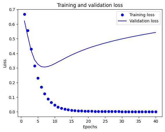
plt.title('Training and validation loss')
plt.xlabel('Epochs')
plt.ylabel('Loss')
plt.legend()
plt.show()
plt.clf()   # clear figure

plt.plot(epochs, acc, 'bo', label='Training acc')
plt.plot(epochs, val_acc, 'b', label='Validation acc')
plt.title('Training and validation accuracy')
plt.xlabel('Epochs')
plt.ylabel('Accuracy')
plt.legend()

plt.show()

このグラフでは、点はトレーニングの損失と正解度を表し、実線は検証の損失と正解度を表します。
トレーニングの損失がエポックごとに下降し、トレーニングの正解度がエポックごとに上昇していることに注目してください。これは、勾配下降最適化を使用しているときに見られる現象で、イテレーションごとに希望する量を最小化します。
これは検証の損失と精度には当てはまりません。20 エポック当たりでピークに達しているようです。これが過適合の例で、モデルが、遭遇したことのないデータよりもトレーニングデータで優れたパフォーマンスを発揮する現象です。この後、モデルは過度に最適化し、テストデータに一般化しないトレーニングデータ特有の表現を学習します。
このような特定のケースについては、約 20 エポック以降のトレーニングを単に停止することで、過適合を回避することができます。この処理をコールバックによって自動的に行う方法については、別の記事で説明します。
# MIT License
#
# Copyright (c) 2017 François Chollet                                  # IGNORE_COPYRIGHT: cleared by OSS licensing
#
# Permission is hereby granted, free of charge, to any person obtaining a
# copy of this software and associated documentation files (the "Software"),
# to deal in the Software without restriction, including without limitation
# the rights to use, copy, modify, merge, publish, distribute, sublicense,
# and/or sell copies of the Software, and to permit persons to whom the
# Software is furnished to do so, subject to the following conditions:
#
# The above copyright notice and this permission notice shall be included in
# all copies or substantial portions of the Software.
#
# THE SOFTWARE IS PROVIDED "AS IS", WITHOUT WARRANTY OF ANY KIND, EXPRESS OR
# IMPLIED, INCLUDING BUT NOT LIMITED TO THE WARRANTIES OF MERCHANTABILITY,
# FITNESS FOR A PARTICULAR PURPOSE AND NONINFRINGEMENT. IN NO EVENT SHALL
# THE AUTHORS OR COPYRIGHT HOLDERS BE LIABLE FOR ANY CLAIM, DAMAGES OR OTHER
# LIABILITY, WHETHER IN AN ACTION OF CONTRACT, TORT OR OTHERWISE, ARISING
# FROM, OUT OF OR IN CONNECTION WITH THE SOFTWARE OR THE USE OR OTHER
# DEALINGS IN THE SOFTWARE.