TensorFlow در 14 مه به Google I/O بازگشته است! همین الان ثبت نام کنید

این صفحه به‌وسیله ‏Cloud Translation API‏ ترجمه شده است.

نوت بوک TFP Release Notes (0.12.1)

هدف این نوت بوک این است که به TFP 0.12.1 کمک کند تا از طریق چند قطعه کوچک زنده شود - دموهای کوچکی از چیزهایی که می توانید با TFP به دست آورید.

مشاهده در TensorFlow.org

در Google Colab اجرا شود

مشاهده منبع در GitHub

دانلود دفترچه یادداشت

نصب و واردات

!pip3 install -qU tensorflow==2.4.0 tensorflow_probability==0.12.1 tensorflow-datasets inference_gym

import tensorflow as tf
import tensorflow_probability as tfp
assert '0.12' in tfp.__version__, tfp.__version__
assert '2.4' in tf.__version__, tf.__version__

physical_devices = tf.config.list_physical_devices('CPU')
tf.config.set_logical_device_configuration(
    physical_devices[0],
    [tf.config.LogicalDeviceConfiguration(),
     tf.config.LogicalDeviceConfiguration()])

tfd = tfp.distributions
tfb = tfp.bijectors
tfpk = tfp.math.psd_kernels

import matplotlib.pyplot as plt
import numpy as np
import scipy.interpolate
import IPython
import seaborn as sns
from inference_gym import using_tensorflow as gym
import logging

بیژکتورها

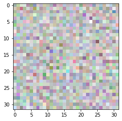
`Glow`

bijector از کاغذ براق: مولد جریان با معکوس 1x1 و پیچش ، توسط کینگما و Dhariwal.

در اینجا نحوه ترسیم تصویر از یک توزیع آمده است (توجه داشته باشید که توزیع در اینجا چیزی "یاد نگرفته است".

image_shape = (32, 32, 4)  # 32 x 32 RGBA image

glow = tfb.Glow(output_shape=image_shape,
                coupling_bijector_fn=tfb.GlowDefaultNetwork,
                exit_bijector_fn=tfb.GlowDefaultExitNetwork)

pz = tfd.Sample(tfd.Normal(0., 1.), tf.reduce_prod(image_shape))

# Calling glow on distribution p(z) creates our glow distribution over images.
px = glow(pz)

# Take samples from the distribution to get images from your dataset.
image = px.sample(1)[0].numpy()

# Rescale to [0, 1].
image = (image - image.min()) / (image.max() - image.min())
plt.imshow(image);

png

`RayleighCDF`

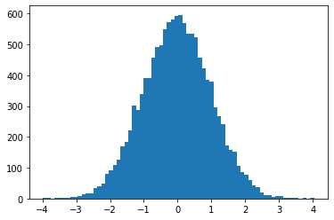
Bijector برای توزیع ریلی CDF. یکی از کاربردها، نمونه برداری از توزیع ریلی، با گرفتن نمونه های یکنواخت، و سپس عبور دادن آنها از معکوس CDF است.

bij = tfb.RayleighCDF()
uniforms = tfd.Uniform().sample(10_000)
plt.hist(bij.inverse(uniforms), bins='auto');

png

`Ascending()` جایگزین `Invert(Ordered())`

x = tfd.Normal(0., 1.).sample(5)
print(tfb.Ascending()(x))
print(tfb.Invert(tfb.Ordered())(x))

tf.Tensor([1.9363368 2.650928  3.4936204 4.1817293 5.6920815], shape=(5,), dtype=float32)
WARNING:tensorflow:From <ipython-input-5-1406b9939c00>:3: Ordered.__init__ (from tensorflow_probability.python.bijectors.ordered) is deprecated and will be removed after 2021-01-09.
Instructions for updating:
`Ordered` bijector is deprecated; please use `tfb.Invert(tfb.Ascending())` instead.
tf.Tensor([1.9363368 2.650928  3.4936204 4.1817293 5.6920815], shape=(5,), dtype=float32)

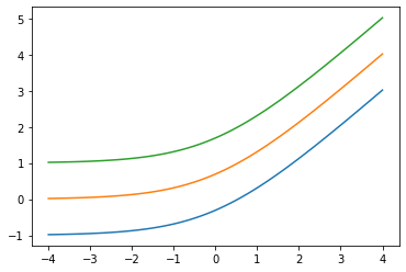
اضافه کردن `low` ارگ: `Softplus(low=2.)`

x = tf.linspace(-4., 4., 100)

for low in (-1., 0., 1.):
  bij = tfb.Softplus(low=low)
  plt.plot(x, bij(x));

png

`tfb.ScaleMatvecLinearOperatorBlock` از blockwise `LinearOperator` ، چند بخشی استدلال

op_1 = tf.linalg.LinearOperatorDiag(diag=[1., -1., 3.])
op_2 = tf.linalg.LinearOperatorFullMatrix([[12., 5.], [-1., 3.]])
scale = tf.linalg.LinearOperatorBlockDiag([op_1, op_2], is_non_singular=True)

bij = tfb.ScaleMatvecLinearOperatorBlock(scale)
bij([[1., 2., 3.], [0., 1.]])

WARNING:tensorflow:From /usr/local/lib/python3.6/dist-packages/tensorflow/python/ops/linalg/linear_operator_block_diag.py:223: LinearOperator.graph_parents (from tensorflow.python.ops.linalg.linear_operator) is deprecated and will be removed in a future version.
Instructions for updating:
Do not call `graph_parents`.
[<tf.Tensor: shape=(3,), dtype=float32, numpy=array([ 1., -2.,  9.], dtype=float32)>,
 <tf.Tensor: shape=(2,), dtype=float32, numpy=array([5., 3.], dtype=float32)>]

توزیع ها

`Skellam`

توزیع بیش از اختلاف دو Poisson RV ها. توجه داشته باشید که نمونه های این توزیع می توانند منفی باشند.

x = tf.linspace(-5., 10., 10 - -5 + 1)

rates = (4, 2)
for i, rate in enumerate(rates):
  plt.bar(x - .3 * (1 - i), tfd.Poisson(rate).prob(x), label=f'Poisson({rate})', alpha=0.5, width=.3)
plt.bar(x.numpy() + .3, tfd.Skellam(*rates).prob(x).numpy(), color='k', alpha=0.25, width=.3,
        label=f'Skellam{rates}')

plt.legend();

png

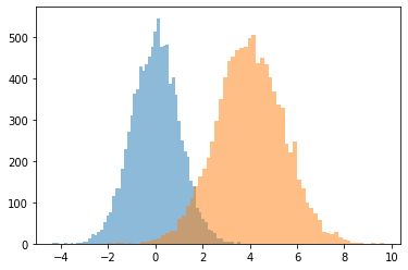
`JointDistributionCoroutine[AutoBatched]` تولید `namedtuple` مانند نمونه

به صراحت مشخص sample_dtype=[...] برای قدیمی tuple رفتار.

@tfd.JointDistributionCoroutineAutoBatched
def model():
  x = yield tfd.Normal(0., 1., name='x')
  y = x + 4.
  yield tfd.Normal(y, 1., name='y')

draw = model.sample(10_000)

plt.hist(draw.x, bins='auto', alpha=0.5)
plt.hist(draw.y, bins='auto', alpha=0.5);

WARNING:tensorflow:Note that RandomStandardNormal inside pfor op may not give same output as inside a sequential loop.
WARNING:tensorflow:Note that RandomStandardNormal inside pfor op may not give same output as inside a sequential loop.

png

`VonMisesFisher` حمایت `dim > 5` ، `entropy()`

توزیع فون میزس-فیشر یک توزیع بر است \(n-1\) حوزه بعدی در \(\mathbb{R}^n\).

dist = tfd.VonMisesFisher([0., 1, 0, 1, 0, 1], concentration=1.)
draws = dist.sample(3)

print(dist.entropy())
tf.reduce_sum(draws ** 2, axis=1)  # each draw has length 1

tf.Tensor(3.3533673, shape=(), dtype=float32)
<tf.Tensor: shape=(3,), dtype=float32, numpy=array([1.0000002 , 0.99999994, 1.0000001 ], dtype=float32)>

`ExpGamma` ، `ExpInverseGamma`

log_rate پارامتر به آن اضافه Gamma . بهبود عددی که نمونه برداری، غلظت کم Beta ، Dirichlet و دوستان. گرادیان های پارامترسازی مجدد ضمنی در همه موارد.

plt.figure(figsize=(10, 3))
plt.subplot(121)
plt.hist(tfd.Beta(.02, .02).sample(10_000), bins='auto')
plt.title('Beta(.02, .02)')
plt.subplot(122)
plt.title('GamX/(GamX+GamY) [the old way]')
g = tfd.Gamma(.02, 1); s0, s1 = g.sample(10_000), g.sample(10_000)
plt.hist(s0 / (s0 + s1), bins='auto')
plt.show()

plt.figure(figsize=(10, 3))
plt.subplot(121)
plt.hist(tfd.ExpGamma(.02, 1.).sample(10_000), bins='auto')
plt.title('ExpGamma(.02, 1)')
plt.subplot(122)
plt.hist(tfb.Log()(tfd.Gamma(.02, 1.)).sample(10_000), bins='auto')
plt.title('tfb.Log()(Gamma(.02, 1)) [the old way]');

png

`JointDistribution*AutoBatched` حمایت نمونه های تجدید پذیر (با طول 2 تایی / دانه تانسور)

@tfd.JointDistributionCoroutineAutoBatched
def model():
  x = yield tfd.Normal(0, 1, name='x')
  y = yield tfd.Normal(x + 4, 1, name='y')

print(model.sample(seed=(1, 2)))
print(model.sample(seed=(1, 2)))

StructTuple(
  x=<tf.Tensor: shape=(), dtype=float32, numpy=-0.59835213>,
  y=<tf.Tensor: shape=(), dtype=float32, numpy=6.2380724>
)
StructTuple(
  x=<tf.Tensor: shape=(), dtype=float32, numpy=-0.59835213>,
  y=<tf.Tensor: shape=(), dtype=float32, numpy=6.2380724>
)

`KL(VonMisesFisher || SphericalUniform)`

# Build vMFs with the same mean direction, batch of increasing concentrations.
vmf = tfd.VonMisesFisher(tf.math.l2_normalize(tf.random.normal([10])),
                         concentration=[0., .1, 1., 10.])
# KL increases with concentration, since vMF(conc=0) == SphericalUniform.
print(tfd.kl_divergence(vmf, tfd.SphericalUniform(10)))

tf.Tensor([4.7683716e-07 4.9877167e-04 4.9384594e-02 2.4844694e+00], shape=(4,), dtype=float32)

`parameter_properties`

کلاس های توزیع در حال حاضر یک معرض parameter_properties(dtype=tf.float32, num_classes=None) روش کلاس، که می تواند ساخت و ساز خودکار از کلاس بسیاری از توزیع های فعال کنید.

print('Gamma:', tfd.Gamma.parameter_properties())
print('Categorical:', tfd.Categorical.parameter_properties(dtype=tf.float64, num_classes=7))

Gamma: {'concentration': ParameterProperties(event_ndims=0, shape_fn=<function ParameterProperties.<lambda> at 0x7ff6bbfcdd90>, default_constraining_bijector_fn=<function Gamma._parameter_properties.<locals>.<lambda> at 0x7ff6afd95510>, is_preferred=True), 'rate': ParameterProperties(event_ndims=0, shape_fn=<function ParameterProperties.<lambda> at 0x7ff6bbfcdd90>, default_constraining_bijector_fn=<function Gamma._parameter_properties.<locals>.<lambda> at 0x7ff6afd95ea0>, is_preferred=False), 'log_rate': ParameterProperties(event_ndims=0, shape_fn=<function ParameterProperties.<lambda> at 0x7ff6bbfcdd90>, default_constraining_bijector_fn=<class 'tensorflow_probability.python.bijectors.identity.Identity'>, is_preferred=True)}
Categorical: {'logits': ParameterProperties(event_ndims=1, shape_fn=<function Categorical._parameter_properties.<locals>.<lambda> at 0x7ff6afd95510>, default_constraining_bijector_fn=<class 'tensorflow_probability.python.bijectors.identity.Identity'>, is_preferred=True), 'probs': ParameterProperties(event_ndims=1, shape_fn=<function Categorical._parameter_properties.<locals>.<lambda> at 0x7ff6afdc91e0>, default_constraining_bijector_fn=<class 'tensorflow_probability.python.bijectors.softmax_centered.SoftmaxCentered'>, is_preferred=False)}

`experimental_default_event_space_bijector`

اکنون آرگ های اضافی را می پذیرد که برخی از قطعات توزیع را سنجاق کند.

@tfd.JointDistributionCoroutineAutoBatched
def model():
  scale = yield tfd.Gamma(1, 1, name='scale')
  obs = yield tfd.Normal(0, scale, name='obs')

model.experimental_default_event_space_bijector(obs=.2).forward(
    [tf.random.uniform([3], -2, 2.)])

StructTuple(
  scale=<tf.Tensor: shape=(3,), dtype=float32, numpy=array([0.6630705, 1.5401832, 1.0777743], dtype=float32)>
)

`JointDistribution.experimental_pin`

پن برخی از بخش توزیع مشترک، بازگشت JointDistributionPinned شی به نمایندگی از تراکم unnormalized مشترک.

کار با experimental_default_event_space_bijector ، این باعث می شود انجام استنتاج تغییرات و یا MCMC با پیش فرض معقول خیلی ساده. در زیر مثال، دو خط اول از sample را در حال اجرا MCMC نسیم.

dist = tfd.JointDistributionSequential([
    tfd.HalfNormal(1.),
    lambda scale: tfd.Normal(0., scale, name='observed')])

@tf.function
def sample():
  bij = dist.experimental_default_event_space_bijector(observed=1.)
  target_log_prob = dist.experimental_pin(observed=1.).unnormalized_log_prob

  kernel = tfp.mcmc.TransformedTransitionKernel(
      tfp.mcmc.HamiltonianMonteCarlo(target_log_prob,
                                     step_size=0.6,
                                     num_leapfrog_steps=16),
      bijector=bij)
  return tfp.mcmc.sample_chain(500, 
                               current_state=tf.ones([8]),  # multiple chains
                               kernel=kernel,
                               trace_fn=None)

draws = sample()

fig, (hist, trace) = plt.subplots(ncols=2, figsize=(16, 3))
trace.plot(draws, alpha=0.5)
for col in tf.transpose(draws):
  sns.kdeplot(col, ax=hist);

png

`tfd.NegativeBinomial.experimental_from_mean_dispersion`

پارامترسازی جایگزین به tfprobability@tensorflow.org ایمیل بزنید یا یک PR برای ما ارسال کنید تا روش‌های کلاس مشابه را برای توزیع‌های دیگر اضافه کنیم.

nb = tfd.NegativeBinomial.experimental_from_mean_dispersion(30., .01)
plt.hist(nb.sample(10_000), bins='auto');

png

`tfp.experimental.distribute`

DistributionStrategy -aware توزیع مشترک، اجازه می دهد برای محاسبات احتمال متقابل دستگاه. Sharded Independent و Sample توزیع.

# Note: 2-logical devices are configured in the install/import cell at top.
strategy = tf.distribute.MirroredStrategy()
assert strategy.num_replicas_in_sync == 2

@tfp.experimental.distribute.JointDistributionCoroutine
def model():
  root = tfp.experimental.distribute.JointDistributionCoroutine.Root
  group_scale = yield root(tfd.Sample(tfd.Exponential(1), 3, name='group_scale'))
  _ = yield tfp.experimental.distribute.ShardedSample(tfd.Independent(tfd.Normal(0, group_scale), 1),
                                                      sample_shape=[4], name='x')

seed1, seed2 = tfp.random.split_seed((1, 2))

@tf.function
def sample(seed):
  return model.sample(seed=seed)
xs = strategy.run(sample, (seed1,))
print("""
Note that the global latent `group_scale` is shared across devices, whereas
the local `x` is sampled independently on each device.
""")
print('sample:', xs)
print('another sample:', strategy.run(sample, (seed2,)))

@tf.function
def log_prob(x):
  return model.log_prob(x)
print("""
Note that each device observes the same log_prob (local latent log_probs are
summed across devices).
""")
print('log_prob:', strategy.run(log_prob, (xs,)))

@tf.function
def grad_log_prob(x):
  return tfp.math.value_and_gradient(model.log_prob, x)[1]

print("""
Note that each device observes the same log_prob gradient (local latents have
independent gradients, global latents have gradients aggregated across devices).
""")
print('grad_log_prob:', strategy.run(grad_log_prob, (xs,)))

WARNING:tensorflow:There are non-GPU devices in `tf.distribute.Strategy`, not using nccl allreduce.
INFO:tensorflow:Using MirroredStrategy with devices ('/job:localhost/replica:0/task:0/device:CPU:0', '/job:localhost/replica:0/task:0/device:CPU:1')

Note that the global latent `group_scale` is shared across devices, whereas 
the local `x` is sampled independently on each device.

sample: StructTuple(
  group_scale=PerReplica:{
      0: <tf.Tensor: shape=(3,), dtype=float32, numpy=array([2.6355493, 1.1805456, 1.245112 ], dtype=float32)>,
      1: <tf.Tensor: shape=(3,), dtype=float32, numpy=array([2.6355493, 1.1805456, 1.245112 ], dtype=float32)>
    },
  x=PerReplica:{
      0: <tf.Tensor: shape=(2, 3), dtype=float32, numpy=
    array([[-0.90548456,  0.7675636 ,  0.27627748],
           [-0.3475989 ,  2.0194046 , -1.2531326 ]], dtype=float32)>,
      1: <tf.Tensor: shape=(2, 3), dtype=float32, numpy=
    array([[ 3.251305  , -0.5790973 ,  0.42745453],
           [-1.562331  ,  0.3006323 ,  0.635732  ]], dtype=float32)>
    }
)
another sample: StructTuple(
  group_scale=PerReplica:{
      0: <tf.Tensor: shape=(3,), dtype=float32, numpy=array([2.41133   , 0.10307606, 0.5236566 ], dtype=float32)>,
      1: <tf.Tensor: shape=(3,), dtype=float32, numpy=array([2.41133   , 0.10307606, 0.5236566 ], dtype=float32)>
    },
  x=PerReplica:{
      0: <tf.Tensor: shape=(2, 3), dtype=float32, numpy=
    array([[-3.2476294 ,  0.07213175, -0.39536062],
           [-1.2319602 , -0.05505352,  0.06356457]], dtype=float32)>,
      1: <tf.Tensor: shape=(2, 3), dtype=float32, numpy=
    array([[ 5.6028705 ,  0.11919801, -0.48446828],
           [-1.5938259 ,  0.21123725,  0.28979057]], dtype=float32)>
    }
)

Note that each device observes the same log_prob (local latent log_probs are
summed across devices).

INFO:tensorflow:Reduce to /job:localhost/replica:0/task:0/device:CPU:0 then broadcast to ('/job:localhost/replica:0/task:0/device:CPU:0', '/job:localhost/replica:0/task:0/device:CPU:1').
log_prob: PerReplica:{
  0: tf.Tensor(-25.05747, shape=(), dtype=float32),
  1: tf.Tensor(-25.05747, shape=(), dtype=float32)
}

Note that each device observes the same log_prob gradient (local latents have
independent gradients, global latents are aggregated across devices).

INFO:tensorflow:Reduce to /job:localhost/replica:0/task:0/device:CPU:0 then broadcast to ('/job:localhost/replica:0/task:0/device:CPU:0', '/job:localhost/replica:0/task:0/device:CPU:1').
INFO:tensorflow:Reduce to /job:localhost/replica:0/task:0/device:CPU:0 then broadcast to ('/job:localhost/replica:0/task:0/device:CPU:0', '/job:localhost/replica:0/task:0/device:CPU:1').
grad_log_prob: StructTuple(
  group_scale=PerReplica:{
      0: <tf.Tensor: shape=(3,), dtype=float32, numpy=array([-1.7555585, -1.2928739, -3.0554674], dtype=float32)>,
      1: <tf.Tensor: shape=(3,), dtype=float32, numpy=array([-1.7555585, -1.2928739, -3.0554674], dtype=float32)>
    },
  x=PerReplica:{
      0: <tf.Tensor: shape=(2, 3), dtype=float32, numpy=
    array([[ 0.13035832, -0.5507428 , -0.17820862],
           [ 0.05004217, -1.4489648 ,  0.80831426]], dtype=float32)>,
      1: <tf.Tensor: shape=(2, 3), dtype=float32, numpy=
    array([[-0.46807498,  0.41551432, -0.27572307],
           [ 0.22492138, -0.21570992, -0.41006932]], dtype=float32)>
    }
)

هسته های PSD

`GeneralizedMatern`

GeneralizedMatern مثبت semidefinite هسته عام MaternOneHalf ، MAterhThreeHalves و MaternFiveHalves .

gm = tfpk.GeneralizedMatern(df=[0.5, 1.5, 2.5], length_scale=1., amplitude=0.5)
m1 = tfpk.MaternOneHalf(length_scale=1., amplitude=0.5)
m2 = tfpk.MaternThreeHalves(length_scale=1., amplitude=0.5)
m3 = tfpk.MaternFiveHalves(length_scale=1., amplitude=0.5)
xs = tf.linspace(-1.5, 1.5, 100)

gm_matrix = gm.matrix([[0.]], xs[..., tf.newaxis])
plt.plot(xs, gm_matrix[0][0])
plt.plot(xs, m1.matrix([[0.]], xs[..., tf.newaxis])[0])
plt.show()
plt.plot(xs, gm_matrix[1][0])
plt.plot(xs, m2.matrix([[0.]], xs[..., tf.newaxis])[0])
plt.show()
plt.plot(xs, gm_matrix[2][0])
plt.plot(xs, m3.matrix([[0.]], xs[..., tf.newaxis])[0])
plt.show()

png

`Parabolic` (Epanechnikov)

epa = tfpk.Parabolic()
xs = tf.linspace(-1.05, 1.05, 100)
plt.plot(xs, epa.matrix([[0.]], xs[..., tf.newaxis])[0]);

png

VI

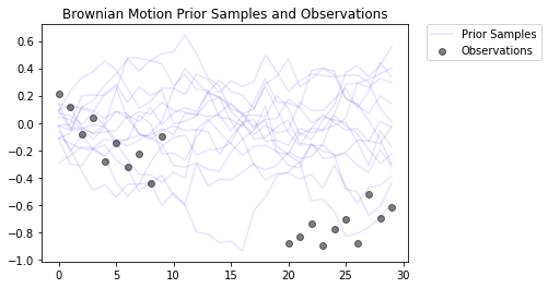
`build_asvi_surrogate_posterior`

به طور خودکار یک جانشین ساختار یافته برای VI بسازید به نحوی که ساختار گرافیکی توزیع قبلی را در خود جای دهد. این بهره گیری از روش شرح داده شده در این مقاله به صورت خودکار ساختار متغیر استنتاج ( https://arxiv.org/abs/2002.00643 ).

# Import a Brownian Motion model from TFP's inference gym.
model = gym.targets.BrownianMotionMissingMiddleObservations()
prior = model.prior_distribution()
ground_truth = ground_truth = model.sample_transformations['identity'].ground_truth_mean
target_log_prob = lambda *values: model.log_likelihood(values) + prior.log_prob(values)

این یک فرآیند حرکت براونی را با یک مدل مشاهده گاوسی مدل می کند. از 30 گام تشکیل شده است، اما 10 گام میانی قابل مشاهده نیستند.

  locs[0] ~ Normal(loc=0, scale=innovation_noise_scale)
  for t in range(1, num_timesteps):
    locs[t] ~ Normal(loc=locs[t - 1], scale=innovation_noise_scale)

  for t in range(num_timesteps):
    observed_locs[t] ~ Normal(loc=locs[t], scale=observation_noise_scale)

هدف این است که برای پی بردن به ارزش های locs از مشاهدات پر سر و صدا ( observed_locs ). از اواسط 10 timesteps غیر قابل مشاهده هستند، observed_locs هستند NaN ارزش ها در timesteps [10،19].

# The observed loc values in the Brownian Motion inference gym model
OBSERVED_LOC = np.array([
    0.21592641, 0.118771404, -0.07945447, 0.037677474, -0.27885845, -0.1484156,
    -0.3250906, -0.22957903, -0.44110894, -0.09830782, np.nan, np.nan, np.nan,
    np.nan, np.nan, np.nan, np.nan, np.nan, np.nan, np.nan, -0.8786016,
    -0.83736074, -0.7384849, -0.8939254, -0.7774566, -0.70238715, -0.87771565,
    -0.51853573, -0.6948214, -0.6202789
]).astype(dtype=np.float32)

# Plot the prior and the likelihood observations
plt.figure()
plt.title('Brownian Motion Prior Samples and Observations')

num_samples = 15
prior_samples = prior.sample(num_samples)

plt.plot(prior_samples, c='blue', alpha=0.1)
plt.plot(prior_samples[0][0], label="Prior Samples", c='blue', alpha=0.1)

plt.scatter(x=range(30),y=OBSERVED_LOC, c='black', alpha=0.5, label="Observations")

plt.legend(bbox_to_anchor=(1.05, 1), borderaxespad=0.);

png

logging.getLogger('tensorflow').setLevel(logging.ERROR)  # suppress pfor warnings

# Construct and train an ASVI Surrogate Posterior.
asvi_surrogate_posterior = tfp.experimental.vi.build_asvi_surrogate_posterior(prior)

asvi_losses = tfp.vi.fit_surrogate_posterior(target_log_prob,
                                        asvi_surrogate_posterior,
                                        optimizer=tf.optimizers.Adam(learning_rate=0.1),
                                        num_steps=500)
logging.getLogger('tensorflow').setLevel(logging.NOTSET)

# Construct and train a Mean-Field Surrogate Posterior.
factored_surrogate_posterior = tfp.experimental.vi.build_factored_surrogate_posterior(event_shape=prior.event_shape)

factored_losses = tfp.vi.fit_surrogate_posterior(target_log_prob,
                                        factored_surrogate_posterior,
                                        optimizer=tf.optimizers.Adam(learning_rate=0.1),
                                        num_steps=500)

logging.getLogger('tensorflow').setLevel(logging.ERROR)  # suppress pfor warnings

# Sample from the posteriors.
asvi_posterior_samples = asvi_surrogate_posterior.sample(num_samples)
factored_posterior_samples = factored_surrogate_posterior.sample(num_samples)

logging.getLogger('tensorflow').setLevel(logging.NOTSET)

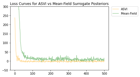
هر دو ASVI و توزیع خلفی جایگزین میدان میانگین همگرا شده‌اند، و ASVI جانشین خلفی از دست دادن نهایی کمتری (مقدار ELBO منفی) داشت.

# Plot the loss curves.
plt.figure()
plt.title('Loss Curves for ASVI vs Mean-Field Surrogate Posteriors')

plt.plot(asvi_losses, c='orange', label='ASVI', alpha = 0.4)
plt.plot(factored_losses, c='green', label='Mean-Field', alpha = 0.4)
plt.ylim(-50, 300)

plt.legend(bbox_to_anchor=(1.3, 1), borderaxespad=0.);

png

نمونه‌های پسین نشان می‌دهند که چگونه خلفی جانشین ASVI به خوبی عدم قطعیت را برای مراحل زمانی بدون مشاهدات ثبت می‌کند. از سوی دیگر، میدان پست جانشین پسینی در تلاش است تا عدم قطعیت واقعی را به تصویر بکشد.

# Plot samples from the ASVI and Mean-Field Surrogate Posteriors.
plt.figure()
plt.title('Posterior Samples from ASVI vs Mean-Field Surrogate Posterior')

plt.plot(asvi_posterior_samples, c='orange', alpha = 0.25)
plt.plot(asvi_posterior_samples[0][0], label='ASVI Surrogate Posterior', c='orange', alpha = 0.25)

plt.plot(factored_posterior_samples, c='green', alpha = 0.25)
plt.plot(factored_posterior_samples[0][0], label='Mean-Field Surrogate Posterior', c='green', alpha = 0.25)

plt.scatter(x=range(30),y=OBSERVED_LOC, c='black', alpha=0.5, label='Observations')

plt.plot(ground_truth, c='black', label='Ground Truth')

plt.legend(bbox_to_anchor=(1.585, 1), borderaxespad=0.);

png

MCMC

`ProgressBarReducer`

پیشرفت نمونه‌گیر را تجسم کنید. (ممکن است جریمه عملکرد اسمی داشته باشد؛ در حال حاضر تحت کامپایل JIT پشتیبانی نمی شود.)

kernel = tfp.mcmc.HamiltonianMonteCarlo(lambda x: -x**2 / 2, .05, 20)
pbar = tfp.experimental.mcmc.ProgressBarReducer(100)
kernel = tfp.experimental.mcmc.WithReductions(kernel, pbar)
plt.hist(tf.reshape(tfp.mcmc.sample_chain(100, current_state=tf.ones([128]), kernel=kernel, trace_fn=None), [-1]), bins='auto')
pbar.bar.close()

99%|█████████▉| 99/100 [00:03<00:00, 27.37it/s]

png

`sample_sequential_monte_carlo` از نمونه های تجدید پذیر

initial_state = tf.random.uniform([4096], -2., 2.)
def smc(seed):
  return tfp.experimental.mcmc.sample_sequential_monte_carlo(
    prior_log_prob_fn=lambda x: -x**2 / 2,
    likelihood_log_prob_fn=lambda x: -(x-1.)**2 / 2,
    current_state=initial_state,
    seed=seed)[1]
plt.hist(smc(seed=(12, 34)), bins='auto');plt.show()

print(smc(seed=(12, 34))[:10])
print('different:', smc(seed=(10, 20))[:10])
print('same:', smc(seed=(12, 34))[:10])

png

tf.Tensor(
[ 0.665834    0.9892149   0.7961128   1.0016634  -1.000767   -0.19461267
  1.3070581   1.127177    0.9940303   0.58239716], shape=(10,), dtype=float32)
different: tf.Tensor(
[ 1.3284367   0.4374407   1.1349089   0.4557473   0.06510283 -0.08954388
  1.1735026   0.8170528   0.12443061  0.34413314], shape=(10,), dtype=float32)
same: tf.Tensor(
[ 0.665834    0.9892149   0.7961128   1.0016634  -1.000767   -0.19461267
  1.3070581   1.127177    0.9940303   0.58239716], shape=(10,), dtype=float32)

اضافه شدن محاسبات جریان واریانس، کوواریانس، Rhat

توجه داشته باشید، رابط به این تا حدودی در تغییر کرده tfp-nightly .

def cov_to_ellipse(t, cov, mean):
  """Draw a one standard deviation ellipse from the mean, according to cov."""
  diag = tf.linalg.diag_part(cov)
  a = 0.5 * tf.reduce_sum(diag)
  b = tf.sqrt(0.25 * (diag[0] - diag[1])**2 + cov[0, 1]**2)
  major = a + b
  minor = a - b
  theta = tf.math.atan2(major - cov[0, 0], cov[0, 1])
  x = (tf.sqrt(major) * tf.cos(theta) * tf.cos(t) -
       tf.sqrt(minor) * tf.sin(theta) * tf.sin(t))
  y = (tf.sqrt(major) * tf.sin(theta) * tf.cos(t) +
       tf.sqrt(minor) * tf.cos(theta) * tf.sin(t))
  return x + mean[0], y + mean[1]

fig, axes = plt.subplots(nrows=4, ncols=5, figsize=(14, 8), 
                         sharex=True, sharey=True, constrained_layout=True)
t = tf.linspace(0., 2 * np.pi, 200)
tot = 10
cov = 0.1 * tf.eye(2) + 0.9 * tf.ones([2, 2])
mvn = tfd.MultivariateNormalTriL(loc=[1., 2.],
                                 scale_tril=tf.linalg.cholesky(cov))

for ax in axes.ravel():
  rv = tfp.experimental.stats.RunningCovariance(
      num_samples=0., mean=tf.zeros(2), sum_squared_residuals=tf.zeros((2, 2)),
      event_ndims=1)

  for idx, x in enumerate(mvn.sample(tot)):
    rv = rv.update(x)
    ax.plot(*cov_to_ellipse(t, rv.covariance(), rv.mean),
            color='k', alpha=(idx + 1) / tot)
  ax.plot(*cov_to_ellipse(t, mvn.covariance(), mvn.mean()), 'r')
fig.suptitle("Twenty tries to approximate the red covariance with 10 draws");

png

ریاضی، آمار

توابع بسل: ive، kve، log-ive

xs = tf.linspace(0.5, 20., 100)
ys = tfp.math.bessel_ive([[0.5], [1.], [np.pi], [4.]], xs)
zs = tfp.math.bessel_kve([[0.5], [1.], [2.], [np.pi]], xs)

for i in range(4):
  plt.plot(xs, ys[i])
plt.show()

for i in range(4):
  plt.plot(xs, zs[i])
plt.show()

png

اختیاری `weights` آرژینین به `tfp.stats.histogram`

edges = tf.linspace(-4., 4, 31)
samps = tfd.TruncatedNormal(0, 1, -4, 4).sample(100_000, seed=(123, 456))
_, (ax1, ax2) = plt.subplots(1, 2, figsize=(10, 3))
ax1.bar(edges[:-1], tfp.stats.histogram(samps, edges))
ax1.set_title('samples histogram')
ax2.bar(edges[:-1], tfp.stats.histogram(samps, edges, weights=1 / tfd.Normal(0, 1).prob(samps)))
ax2.set_title('samples, weighted by inverse p(sample)');

png

`tfp.math.erfcinv`

x = tf.linspace(-3., 3., 10)
y = tf.math.erfc(x)
z = tfp.math.erfcinv(y)
print(x)
print(z)

tf.Tensor(
[-3.         -2.3333333  -1.6666666  -1.         -0.33333325  0.3333335

  1.          1.666667    2.3333335   3.        ], shape=(10,), dtype=float32)
tf.Tensor(
[-3.0002644  -2.3333426  -1.6666666  -0.9999997  -0.3333332   0.33333346
  0.9999999   1.6666667   2.3333335   3.0000002 ], shape=(10,), dtype=float32)

نوت بوک TFP Release Notes (0.12.1)

نصب و واردات

بیژکتورها

Glow

RayleighCDF

Ascending() جایگزین Invert(Ordered())

اضافه کردن low ارگ: Softplus(low=2.)

tfb.ScaleMatvecLinearOperatorBlock از blockwise LinearOperator ، چند بخشی استدلال

توزیع ها

Skellam

JointDistributionCoroutine[AutoBatched] تولید namedtuple مانند نمونه

VonMisesFisher حمایت dim > 5 ، entropy()

ExpGamma ، ExpInverseGamma

JointDistribution*AutoBatched حمایت نمونه های تجدید پذیر (با طول 2 تایی / دانه تانسور)

KL(VonMisesFisher || SphericalUniform)

parameter_properties

experimental_default_event_space_bijector

JointDistribution.experimental_pin

tfd.NegativeBinomial.experimental_from_mean_dispersion

tfp.experimental.distribute