พยากรณ์อนุกรมเวลา

บทช่วยสอนนี้เป็นการแนะนำการพยากรณ์อนุกรมเวลาโดยใช้ TensorFlow มันสร้างรูปแบบที่แตกต่างกันสองสามรูปแบบรวมถึง Convolutional และ Recurrent Neural Networks (CNNs และ RNNs)

นี้ครอบคลุมในสองส่วนหลัก โดยมีส่วนย่อย:

• พยากรณ์สำหรับขั้นตอนเดียว:
  • คุณสมบัติเดียว
  • คุณสมบัติทั้งหมด
• พยากรณ์หลายขั้นตอน:
  • นัดเดียว: ทำนายทั้งหมดพร้อมกัน
  • Autoregressive: ทำนายทีละครั้งและป้อนผลลัพธ์กลับไปยังแบบจำลอง

ติดตั้ง

import os
import datetime

import IPython
import IPython.display
import matplotlib as mpl
import matplotlib.pyplot as plt
import numpy as np
import pandas as pd
import seaborn as sns
import tensorflow as tf

mpl.rcParams['figure.figsize'] = (8, 6)
mpl.rcParams['axes.grid'] = False

ชุดข้อมูลสภาพอากาศ

บทช่วยสอนนี้ใช้ ชุดข้อมูลอนุกรมเวลาสภาพอากาศที่ บันทึกโดย Max Planck Institute for Biogeochemistry

ชุดข้อมูลนี้มีคุณลักษณะต่างๆ 14 อย่าง เช่น อุณหภูมิของอากาศ ความกดอากาศ และความชื้น สิ่งเหล่านี้ถูกรวบรวมทุกๆ 10 นาที เริ่มในปี 2546 เพื่อประสิทธิภาพ คุณจะใช้เฉพาะข้อมูลที่รวบรวมระหว่างปี 2009 ถึง 2016 เท่านั้น ชุดข้อมูลส่วนนี้จัดทำโดย François Chollet สำหรับหนังสือ Deep Learning with Python ของเขา

zip_path = tf.keras.utils.get_file(
    origin='https://storage.googleapis.com/tensorflow/tf-keras-datasets/jena_climate_2009_2016.csv.zip',
    fname='jena_climate_2009_2016.csv.zip',
    extract=True)
csv_path, _ = os.path.splitext(zip_path)

Downloading data from https://storage.googleapis.com/tensorflow/tf-keras-datasets/jena_climate_2009_2016.csv.zip
13574144/13568290 [==============================] - 1s 0us/step
13582336/13568290 [==============================] - 1s 0us/step

บทแนะนำนี้จะจัดการกับ การคาดการณ์รายชั่วโมง ดังนั้นให้เริ่มต้นด้วยการสุ่มตัวอย่างข้อมูลจากช่วงเวลา 10 นาทีถึงช่วงเวลาหนึ่งชั่วโมง:

df = pd.read_csv(csv_path)
# Slice [start:stop:step], starting from index 5 take every 6th record.
df = df[5::6]

date_time = pd.to_datetime(df.pop('Date Time'), format='%d.%m.%Y %H:%M:%S')

มาดูข้อมูลกันก่อน นี่คือสองสามแถวแรก:

df.head()

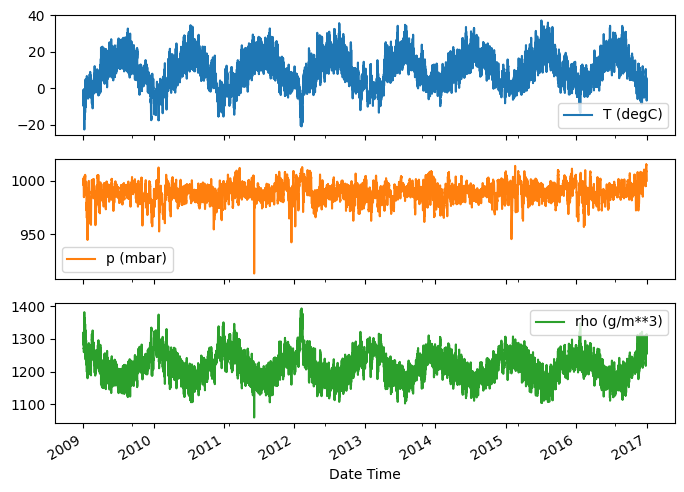
นี่คือวิวัฒนาการของคุณสมบัติบางอย่างเมื่อเวลาผ่านไป:

plot_cols = ['T (degC)', 'p (mbar)', 'rho (g/m**3)']
plot_features = df[plot_cols]
plot_features.index = date_time
_ = plot_features.plot(subplots=True)

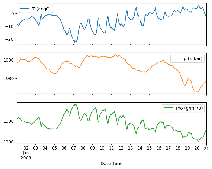
plot_features = df[plot_cols][:480]
plot_features.index = date_time[:480]
_ = plot_features.plot(subplots=True)

ตรวจสอบและทำความสะอาด

ต่อไป ดูสถิติของชุดข้อมูล:

df.describe().transpose()

ความเร็วลม

สิ่งหนึ่งที่ควรโดดเด่นคือค่า min สุดของความเร็วลม ( wv (m/s) ) และค่าสูงสุด ( max. wv (m/s) ) คอลัมน์ -9999 นี้น่าจะผิดพลาด

มีคอลัมน์บอกทิศทางลมแยกต่างหาก ดังนั้นความเร็วควรมากกว่าศูนย์ ( >=0 ) แทนที่ด้วยศูนย์:

wv = df['wv (m/s)']
bad_wv = wv == -9999.0
wv[bad_wv] = 0.0

max_wv = df['max. wv (m/s)']
bad_max_wv = max_wv == -9999.0
max_wv[bad_max_wv] = 0.0

# The above inplace edits are reflected in the DataFrame.
df['wv (m/s)'].min()

0.0

วิศวกรรมคุณลักษณะ

ก่อนดำดิ่งสู่การสร้างแบบจำลอง สิ่งสำคัญคือต้องเข้าใจข้อมูลของคุณ และตรวจสอบให้แน่ใจว่าคุณกำลังส่งข้อมูลที่มีรูปแบบเหมาะสมของแบบจำลอง

ลม

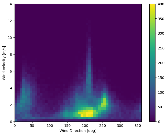
คอลัมน์สุดท้ายของข้อมูล wd (deg) กำหนดทิศทางลมในหน่วยองศา มุมไม่ได้สร้างอินพุตแบบจำลองที่ดี: 360° และ 0° ควรอยู่ใกล้กันและพันรอบอย่างราบรื่น ทิศทางไม่สำคัญถ้าลมไม่พัด

ขณะนี้การกระจายข้อมูลลมมีลักษณะดังนี้:

plt.hist2d(df['wd (deg)'], df['wv (m/s)'], bins=(50, 50), vmax=400)
plt.colorbar()
plt.xlabel('Wind Direction [deg]')
plt.ylabel('Wind Velocity [m/s]')

Text(0, 0.5, 'Wind Velocity [m/s]')

แต่สิ่งนี้จะง่ายกว่าสำหรับแบบจำลองที่จะตีความหากคุณแปลงทิศทางลมและคอลัมน์ความเร็วเป็น เวกเตอร์ ลม :

wv = df.pop('wv (m/s)')
max_wv = df.pop('max. wv (m/s)')

# Convert to radians.
wd_rad = df.pop('wd (deg)')*np.pi / 180

# Calculate the wind x and y components.
df['Wx'] = wv*np.cos(wd_rad)
df['Wy'] = wv*np.sin(wd_rad)

# Calculate the max wind x and y components.
df['max Wx'] = max_wv*np.cos(wd_rad)
df['max Wy'] = max_wv*np.sin(wd_rad)

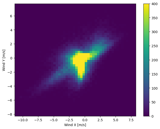
การกระจายเวกเตอร์ลมนั้นง่ายกว่ามากสำหรับแบบจำลองในการตีความอย่างถูกต้อง:

plt.hist2d(df['Wx'], df['Wy'], bins=(50, 50), vmax=400)
plt.colorbar()
plt.xlabel('Wind X [m/s]')
plt.ylabel('Wind Y [m/s]')
ax = plt.gca()
ax.axis('tight')

(-11.305513973134667, 8.24469928549079, -8.27438540335515, 7.7338312955467785)

เวลา

ในทำนองเดียวกัน คอลัมน์ Date Time มีประโยชน์มาก แต่ไม่ใช่ในรูปแบบสตริงนี้ เริ่มต้นด้วยการแปลงเป็นวินาที:

timestamp_s = date_time.map(pd.Timestamp.timestamp)

เช่นเดียวกับทิศทางลม เวลาในหน่วยวินาทีไม่ใช่ข้อมูลโมเดลที่มีประโยชน์ เนื่องจากเป็นข้อมูลสภาพอากาศจึงมีช่วงเวลารายวันและรายปีที่ชัดเจน มีหลายวิธีที่คุณสามารถจัดการกับช่วงเวลาได้

คุณสามารถรับสัญญาณที่ใช้งานได้โดยใช้การแปลงไซน์และโคไซน์เพื่อล้างสัญญาณ "เวลาของวัน" และ "เวลาของปี":

day = 24*60*60
year = (365.2425)*day

df['Day sin'] = np.sin(timestamp_s * (2 * np.pi / day))
df['Day cos'] = np.cos(timestamp_s * (2 * np.pi / day))
df['Year sin'] = np.sin(timestamp_s * (2 * np.pi / year))
df['Year cos'] = np.cos(timestamp_s * (2 * np.pi / year))

plt.plot(np.array(df['Day sin'])[:25])
plt.plot(np.array(df['Day cos'])[:25])
plt.xlabel('Time [h]')
plt.title('Time of day signal')

Text(0.5, 1.0, 'Time of day signal')

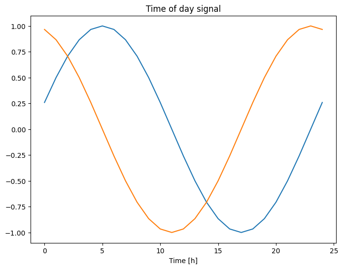
ซึ่งจะทำให้โมเดลเข้าถึงคุณลักษณะความถี่ที่สำคัญที่สุดได้ ในกรณีนี้ คุณจะรู้ล่วงหน้าว่าความถี่ใดมีความสำคัญ

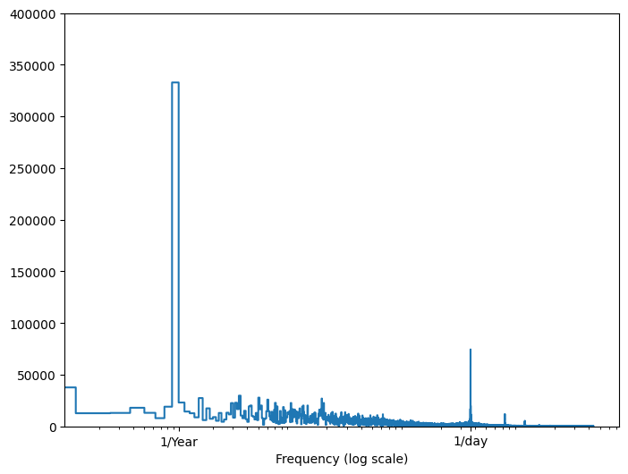
หากคุณไม่มีข้อมูลดังกล่าว คุณสามารถกำหนดความถี่ที่สำคัญได้โดยการแยกคุณลักษณะด้วย Fast Fourier Transform เพื่อตรวจสอบสมมติฐาน นี่คือ tf.signal.rfft ของอุณหภูมิเมื่อเวลาผ่านไป สังเกตพีคที่ชัดเจนที่ความถี่ใกล้ 1/year และ 1/day :

fft = tf.signal.rfft(df['T (degC)'])
f_per_dataset = np.arange(0, len(fft))

n_samples_h = len(df['T (degC)'])
hours_per_year = 24*365.2524
years_per_dataset = n_samples_h/(hours_per_year)

f_per_year = f_per_dataset/years_per_dataset
plt.step(f_per_year, np.abs(fft))
plt.xscale('log')
plt.ylim(0, 400000)
plt.xlim([0.1, max(plt.xlim())])
plt.xticks([1, 365.2524], labels=['1/Year', '1/day'])
_ = plt.xlabel('Frequency (log scale)')

แยกข้อมูล

คุณจะใช้การแบ่ง (70%, 20%, 10%) สำหรับการฝึก การตรวจสอบ และชุดทดสอบ โปรดทราบว่าข้อมูลจะ ไม่ ถูกสุ่มแบบสุ่มก่อนที่จะแยก ด้วยเหตุผลสองประการ:

1. ช่วยให้มั่นใจได้ว่าการสับข้อมูลลงในหน้าต่างของตัวอย่างที่ต่อเนื่องกันยังคงเป็นไปได้
2. ช่วยให้มั่นใจได้ว่าผลการตรวจสอบ/การทดสอบมีความสมจริงมากขึ้น โดยจะได้รับการประเมินจากข้อมูลที่รวบรวมหลังจากฝึกแบบจำลอง

column_indices = {name: i for i, name in enumerate(df.columns)}

n = len(df)
train_df = df[0:int(n*0.7)]
val_df = df[int(n*0.7):int(n*0.9)]
test_df = df[int(n*0.9):]

num_features = df.shape[1]

ทำให้ข้อมูลเป็นปกติ

สิ่งสำคัญคือต้องปรับขนาดคุณสมบัติก่อนฝึกโครงข่ายประสาทเทียม การทำให้เป็นมาตรฐานเป็นวิธีทั่วไปในการปรับขนาดนี้: ลบค่าเฉลี่ยและหารด้วยค่าเบี่ยงเบนมาตรฐานของแต่ละจุดสนใจ

ค่าเฉลี่ยและค่าเบี่ยงเบนมาตรฐานควรคำนวณโดยใช้ข้อมูลการฝึกเท่านั้น เพื่อให้แบบจำลองไม่สามารถเข้าถึงค่าในชุดตรวจสอบและชุดทดสอบได้

นอกจากนี้ยังสามารถโต้แย้งได้ว่าแบบจำลองไม่ควรเข้าถึงค่าในอนาคตในชุดการฝึกเมื่อทำการฝึก และการทำให้เป็นมาตรฐานนี้ควรทำโดยใช้ค่าเฉลี่ยเคลื่อนที่ นั่นไม่ใช่จุดสนใจของบทช่วยสอนนี้ และชุดการตรวจสอบและการทดสอบช่วยให้แน่ใจว่าคุณจะได้รับตัวชี้วัดที่ตรงไปตรงมา (ค่อนข้าง) ดังนั้น เพื่อความเรียบง่าย บทช่วยสอนนี้จึงใช้ค่าเฉลี่ยอย่างง่าย

train_mean = train_df.mean()
train_std = train_df.std()

train_df = (train_df - train_mean) / train_std
val_df = (val_df - train_mean) / train_std
test_df = (test_df - train_mean) / train_std

ตอนนี้ให้ดูที่การกระจายของคุณสมบัติ คุณลักษณะบางอย่างมีหางยาว แต่ไม่มีข้อผิดพลาดที่ชัดเจนเช่นค่าความเร็วลม -9999

df_std = (df - train_mean) / train_std
df_std = df_std.melt(var_name='Column', value_name='Normalized')
plt.figure(figsize=(12, 6))
ax = sns.violinplot(x='Column', y='Normalized', data=df_std)
_ = ax.set_xticklabels(df.keys(), rotation=90)

หน้าต่างข้อมูล

ตัวแบบในบทช่วยสอนนี้จะสร้างชุดการคาดคะเนตามหน้าต่างของตัวอย่างที่ต่อเนื่องกันจากข้อมูล

คุณสมบัติหลักของหน้าต่างอินพุตคือ:

• ความกว้าง (จำนวนขั้นตอนของเวลา) ของหน้าต่างอินพุตและป้ายกำกับ
• เวลาชดเชยระหว่างพวกเขา
• คุณลักษณะใดใช้เป็นอินพุต ป้ายกำกับ หรือทั้งสองอย่าง

บทช่วยสอนนี้สร้างโมเดลที่หลากหลาย (รวมถึงโมเดล Linear, DNN, CNN และ RNN) และใช้สำหรับทั้งสอง:

• เอาต์พุตเดี่ยว และการคาดการณ์ หลายเอาต์พุต
• การทำนายขั้นตอน เดียว และ หลายขั้นตอน

ส่วนนี้เน้นที่การนำหน้าต่างข้อมูลไปใช้ใหม่เพื่อให้สามารถใช้ซ้ำได้กับโมเดลทั้งหมดเหล่านั้น

ขึ้นอยู่กับงานและประเภทของแบบจำลอง คุณอาจต้องการสร้างหน้าต่างข้อมูลที่หลากหลาย นี่คือตัวอย่างบางส่วน:

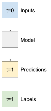
1. ตัวอย่างเช่น หากต้องการคาดการณ์ล่วงหน้า 24 ชั่วโมงในอนาคต โดยระบุประวัติ 24 ชั่วโมง คุณอาจกำหนดหน้าต่างดังนี้:

   

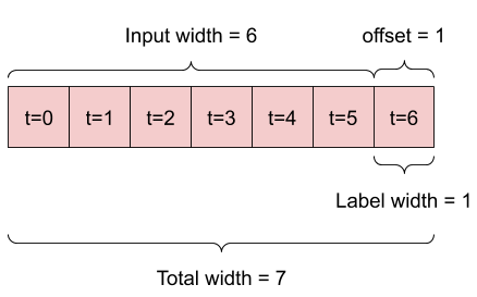
2. แบบจำลองที่ทำนายอนาคตหนึ่งชั่วโมงจากประวัติศาสตร์หกชั่วโมง จะต้องมีหน้าต่างแบบนี้:

   

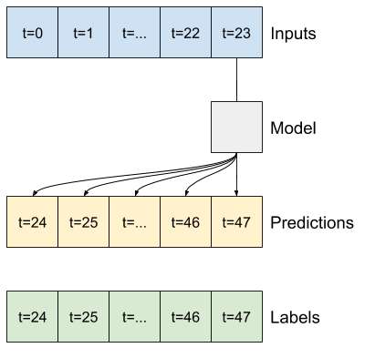
ส่วนที่เหลือของส่วนนี้กำหนดคลาส WindowGenerator ชั้นเรียนนี้สามารถ:

1. จัดการดัชนีและออฟเซ็ตตามที่แสดงในไดอะแกรมด้านบน
2. แบ่งหน้าต่างคุณสมบัติออกเป็นคู่ (features, labels)
3. พล็อตเนื้อหาของหน้าต่างผลลัพธ์
4. สร้างชุดของหน้าต่างเหล่านี้อย่างมีประสิทธิภาพจากข้อมูลการฝึกอบรม การประเมิน และการทดสอบ โดยใช้ tf.data.Dataset

1. ดัชนีและออฟเซ็ต

เริ่มต้นด้วยการสร้างคลาส WindowGenerator เมธอด __init__ รวมตรรกะที่จำเป็นทั้งหมดสำหรับดัชนีอินพุตและป้ายกำกับ

นอกจากนี้ยังใช้การฝึกอบรม ประเมินผล และทดสอบ DataFrames เป็นข้อมูลเข้า สิ่งเหล่านี้จะถูกแปลงเป็น tf.data.Dataset ของ windows ในภายหลัง

class WindowGenerator():
  def __init__(self, input_width, label_width, shift,
               train_df=train_df, val_df=val_df, test_df=test_df,
               label_columns=None):
    # Store the raw data.
    self.train_df = train_df
    self.val_df = val_df
    self.test_df = test_df

    # Work out the label column indices.
    self.label_columns = label_columns
    if label_columns is not None:
      self.label_columns_indices = {name: i for i, name in
                                    enumerate(label_columns)}
    self.column_indices = {name: i for i, name in
                           enumerate(train_df.columns)}

    # Work out the window parameters.
    self.input_width = input_width
    self.label_width = label_width
    self.shift = shift

    self.total_window_size = input_width + shift

    self.input_slice = slice(0, input_width)
    self.input_indices = np.arange(self.total_window_size)[self.input_slice]

    self.label_start = self.total_window_size - self.label_width
    self.labels_slice = slice(self.label_start, None)
    self.label_indices = np.arange(self.total_window_size)[self.labels_slice]

  def __repr__(self):
    return '\n'.join([
        f'Total window size: {self.total_window_size}',
        f'Input indices: {self.input_indices}',
        f'Label indices: {self.label_indices}',
        f'Label column name(s): {self.label_columns}'])

นี่คือรหัสสำหรับสร้าง 2 หน้าต่างที่แสดงในไดอะแกรมที่จุดเริ่มต้นของส่วนนี้:

w1 = WindowGenerator(input_width=24, label_width=1, shift=24,
                     label_columns=['T (degC)'])
w1

Total window size: 48
Input indices: [ 0  1  2  3  4  5  6  7  8  9 10 11 12 13 14 15 16 17 18 19 20 21 22 23]
Label indices: [47]
Label column name(s): ['T (degC)']

w2 = WindowGenerator(input_width=6, label_width=1, shift=1,
                     label_columns=['T (degC)'])
w2

Total window size: 7
Input indices: [0 1 2 3 4 5]
Label indices: [6]
Label column name(s): ['T (degC)']

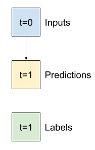
2. แยก

เมื่อระบุรายการอินพุตที่ต่อเนื่องกัน วิธี split_window จะแปลงเป็นหน้าต่างอินพุตและหน้าต่างป้ายกำกับ

ตัวอย่าง w2 ที่คุณกำหนดไว้ก่อนหน้านี้จะถูกแบ่งดังนี้:

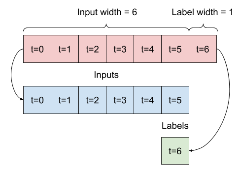
ไดอะแกรมนี้ไม่แสดงแกน features ของข้อมูล แต่ฟังก์ชัน split_window นี้ยังจัดการ label_columns เพื่อให้สามารถใช้ได้กับทั้งตัวอย่างเอาต์พุตเดี่ยวและหลายเอาต์พุต

def split_window(self, features):
  inputs = features[:, self.input_slice, :]
  labels = features[:, self.labels_slice, :]
  if self.label_columns is not None:
    labels = tf.stack(
        [labels[:, :, self.column_indices[name]] for name in self.label_columns],
        axis=-1)

  # Slicing doesn't preserve static shape information, so set the shapes
  # manually. This way the `tf.data.Datasets` are easier to inspect.
  inputs.set_shape([None, self.input_width, None])
  labels.set_shape([None, self.label_width, None])

  return inputs, labels

WindowGenerator.split_window = split_window

ลองใช้:

# Stack three slices, the length of the total window.
example_window = tf.stack([np.array(train_df[:w2.total_window_size]),
                           np.array(train_df[100:100+w2.total_window_size]),
                           np.array(train_df[200:200+w2.total_window_size])])

example_inputs, example_labels = w2.split_window(example_window)

print('All shapes are: (batch, time, features)')
print(f'Window shape: {example_window.shape}')
print(f'Inputs shape: {example_inputs.shape}')
print(f'Labels shape: {example_labels.shape}')

All shapes are: (batch, time, features)
Window shape: (3, 7, 19)
Inputs shape: (3, 6, 19)
Labels shape: (3, 1, 1)

โดยทั่วไป ข้อมูลใน TensorFlow จะถูกบรรจุลงในอาร์เรย์โดยที่ดัชนีที่อยู่นอกสุดข้ามตัวอย่าง (มิติ "แบทช์") ดัชนีกลางคือมิติข้อมูล "เวลา" หรือ "ช่องว่าง" (ความกว้าง ความสูง) ดัชนีในสุดคือคุณสมบัติ

โค้ดด้านบนใช้หน้าต่างขั้นตอน 7 เวลาสามชุดพร้อมฟีเจอร์ 19 รายการในแต่ละขั้นตอน โดยแบ่งออกเป็นชุดอินพุตคุณสมบัติ 19 ขั้นตอน 6 ครั้ง และเลเบลคุณสมบัติขั้นตอนที่ 1 1 ครั้ง ป้ายกำกับมีคุณลักษณะเดียวเท่านั้นเนื่องจาก WindowGenerator เริ่มต้นด้วย label_columns=['T (degC)'] ในขั้นต้น บทช่วยสอนนี้จะสร้างแบบจำลองที่คาดการณ์ป้ายกำกับเอาต์พุตเดี่ยว

3. พล็อต

นี่คือวิธีการลงจุดที่ช่วยให้มองเห็นภาพอย่างง่ายของหน้าต่างแยก:

w2.example = example_inputs, example_labels

def plot(self, model=None, plot_col='T (degC)', max_subplots=3):
  inputs, labels = self.example
  plt.figure(figsize=(12, 8))
  plot_col_index = self.column_indices[plot_col]
  max_n = min(max_subplots, len(inputs))
  for n in range(max_n):
    plt.subplot(max_n, 1, n+1)
    plt.ylabel(f'{plot_col} [normed]')
    plt.plot(self.input_indices, inputs[n, :, plot_col_index],
             label='Inputs', marker='.', zorder=-10)

    if self.label_columns:
      label_col_index = self.label_columns_indices.get(plot_col, None)
    else:
      label_col_index = plot_col_index

    if label_col_index is None:
      continue

    plt.scatter(self.label_indices, labels[n, :, label_col_index],
                edgecolors='k', label='Labels', c='#2ca02c', s=64)
    if model is not None:
      predictions = model(inputs)
      plt.scatter(self.label_indices, predictions[n, :, label_col_index],
                  marker='X', edgecolors='k', label='Predictions',
                  c='#ff7f0e', s=64)

    if n == 0:
      plt.legend()

  plt.xlabel('Time [h]')

WindowGenerator.plot = plot

ตัวยึดตำแหน่ง32

พล็อตนี้จัดแนวอินพุต ป้ายกำกับ และการคาดการณ์ (ภายหลัง) ตามเวลาที่รายการอ้างอิงถึง:

w2.plot()

คุณสามารถพล็อตคอลัมน์อื่นๆ ได้ แต่การกำหนดค่าหน้าต่าง w2 ตัวอย่างมีป้ายกำกับสำหรับคอลัมน์ T (degC) เท่านั้น

w2.plot(plot_col='p (mbar)')

4. สร้าง tf.data.Dataset s

สุดท้าย เมธอด make_dataset นี้จะใช้ DataFrame อนุกรมเวลาและแปลงเป็น tf.data.Dataset ของคู่ (input_window, label_window) โดยใช้ฟังก์ชัน tf.keras.utils.timeseries_dataset_from_array :

def make_dataset(self, data):
  data = np.array(data, dtype=np.float32)
  ds = tf.keras.utils.timeseries_dataset_from_array(
      data=data,
      targets=None,
      sequence_length=self.total_window_size,
      sequence_stride=1,
      shuffle=True,
      batch_size=32,)

  ds = ds.map(self.split_window)

  return ds

WindowGenerator.make_dataset = make_dataset

วัตถุ WindowGenerator เก็บข้อมูลการฝึกอบรม การตรวจสอบ และการทดสอบ

เพิ่มคุณสมบัติสำหรับการเข้าถึงเป็น tf.data.Dataset โดยใช้เมธอด make_dataset ที่คุณกำหนดไว้ก่อนหน้านี้ เพิ่มชุดตัวอย่างมาตรฐานเพื่อให้เข้าถึงและวางแผนได้ง่าย:

@property
def train(self):
  return self.make_dataset(self.train_df)

@property
def val(self):
  return self.make_dataset(self.val_df)

@property
def test(self):
  return self.make_dataset(self.test_df)

@property
def example(self):
  """Get and cache an example batch of `inputs, labels` for plotting."""
  result = getattr(self, '_example', None)
  if result is None:
    # No example batch was found, so get one from the `.train` dataset
    result = next(iter(self.train))
    # And cache it for next time
    self._example = result
  return result

WindowGenerator.train = train
WindowGenerator.val = val
WindowGenerator.test = test
WindowGenerator.example = example

ตอนนี้อ็อบเจ็กต์ WindowGenerator ให้คุณเข้าถึง tf.data.Dataset ดังนั้นคุณจึงสามารถวนซ้ำข้อมูลได้อย่างง่ายดาย

คุณสมบัติ Dataset.element_spec จะบอกคุณถึงโครงสร้าง ชนิดข้อมูล และรูปร่างขององค์ประกอบชุดข้อมูล

# Each element is an (inputs, label) pair.
w2.train.element_spec

(TensorSpec(shape=(None, 6, 19), dtype=tf.float32, name=None),
 TensorSpec(shape=(None, 1, 1), dtype=tf.float32, name=None))

การวนซ้ำ Dataset ทำให้เกิดแบตช์ที่เป็นรูปธรรม:

for example_inputs, example_labels in w2.train.take(1):
  print(f'Inputs shape (batch, time, features): {example_inputs.shape}')
  print(f'Labels shape (batch, time, features): {example_labels.shape}')

Inputs shape (batch, time, features): (32, 6, 19)
Labels shape (batch, time, features): (32, 1, 1)

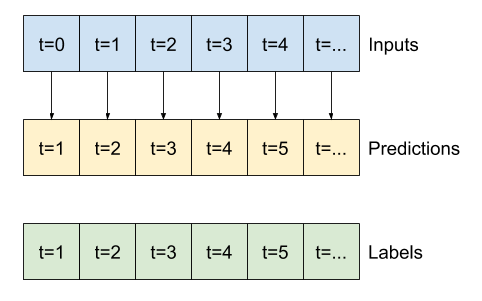
รุ่นขั้นตอนเดียว

โมเดลที่ง่ายที่สุดที่คุณสามารถสร้างจากข้อมูลประเภทนี้ได้คือโมเดลที่คาดการณ์คุณค่าของคุณลักษณะเดียว—ขั้นตอนเวลา 1 ครั้ง (หนึ่งชั่วโมง) ในอนาคตโดยอิงตามเงื่อนไขปัจจุบันเท่านั้น

ดังนั้น ให้เริ่มต้นด้วยการสร้างแบบจำลองเพื่อทำนายค่า T (degC) ในอีกหนึ่งชั่วโมงข้างหน้า

กำหนดค่าอ็อบเจ็กต์ WindowGenerator เพื่อสร้างคู่ขั้นตอนเดียว (input, label) เหล่านี้:

single_step_window = WindowGenerator(
    input_width=1, label_width=1, shift=1,
    label_columns=['T (degC)'])
single_step_window

Total window size: 2
Input indices: [0]
Label indices: [1]
Label column name(s): ['T (degC)']

ตัวยึดตำแหน่ง42

วัตถุ window สร้าง tf.data.Dataset จากชุดการฝึก การตรวจสอบความถูกต้อง และชุดทดสอบ ช่วยให้คุณทำซ้ำชุดข้อมูลได้อย่างง่ายดาย

for example_inputs, example_labels in single_step_window.train.take(1):
  print(f'Inputs shape (batch, time, features): {example_inputs.shape}')
  print(f'Labels shape (batch, time, features): {example_labels.shape}')

Inputs shape (batch, time, features): (32, 1, 19)
Labels shape (batch, time, features): (32, 1, 1)

พื้นฐาน

ก่อนที่จะสร้างแบบจำลองที่ฝึกได้ ควรมีพื้นฐานประสิทธิภาพเป็นจุดในการเปรียบเทียบกับแบบจำลองที่ซับซ้อนกว่าในภายหลัง

งานแรกนี้คือการทำนายอุณหภูมิในอีกหนึ่งชั่วโมงข้างหน้า โดยพิจารณาจากมูลค่าปัจจุบันของคุณสมบัติทั้งหมด ค่าปัจจุบันรวมถึงอุณหภูมิปัจจุบัน

ดังนั้น ให้เริ่มต้นด้วยแบบจำลองที่เพิ่งคืนค่าอุณหภูมิปัจจุบันเป็นการคาดคะเน โดยคาดการณ์ว่า "ไม่มีการเปลี่ยนแปลง" นี่เป็นพื้นฐานที่สมเหตุสมผลเนื่องจากอุณหภูมิเปลี่ยนแปลงช้า แน่นอนว่าเส้นฐานนี้จะทำงานได้ดีน้อยลงหากคุณคาดการณ์เพิ่มเติมในอนาคต

class Baseline(tf.keras.Model):
  def __init__(self, label_index=None):
    super().__init__()
    self.label_index = label_index

  def call(self, inputs):
    if self.label_index is None:
      return inputs
    result = inputs[:, :, self.label_index]
    return result[:, :, tf.newaxis]

สร้างอินสแตนซ์และประเมินโมเดลนี้:

baseline = Baseline(label_index=column_indices['T (degC)'])

baseline.compile(loss=tf.losses.MeanSquaredError(),
                 metrics=[tf.metrics.MeanAbsoluteError()])

val_performance = {}
performance = {}
val_performance['Baseline'] = baseline.evaluate(single_step_window.val)
performance['Baseline'] = baseline.evaluate(single_step_window.test, verbose=0)

439/439 [==============================] - 1s 2ms/step - loss: 0.0128 - mean_absolute_error: 0.0785

ที่พิมพ์เมตริกประสิทธิภาพบางอย่าง แต่สิ่งเหล่านี้ไม่ได้ทำให้คุณรู้สึกว่าโมเดลทำงานได้ดีเพียงใด

WindowGenerator มีวิธีพล็อต แต่พล็อตจะไม่น่าสนใจมากนักด้วยตัวอย่างเพียงตัวอย่างเดียว

ดังนั้น ให้สร้าง WindowGenerator ที่กว้างขึ้นซึ่งสร้างหน้าต่างอินพุตและป้ายกำกับต่อเนื่องกันตลอด 24 ชั่วโมงในแต่ละครั้ง ตัวแปร wide_window ใหม่จะไม่เปลี่ยนวิธีการทำงานของโมเดล โมเดลยังคงคาดการณ์ล่วงหน้าหนึ่งชั่วโมงในอนาคตโดยอิงตามขั้นตอนเวลาอินพุตเดียว ในที่นี้ แกน time จะทำหน้าที่เหมือนแกนของ batch งาน: การคาดคะเนแต่ละรายการถูกสร้างขึ้นอย่างอิสระโดยไม่มีการโต้ตอบระหว่างขั้นตอนของเวลา:

wide_window = WindowGenerator(
    input_width=24, label_width=24, shift=1,
    label_columns=['T (degC)'])

wide_window

Total window size: 25
Input indices: [ 0  1  2  3  4  5  6  7  8  9 10 11 12 13 14 15 16 17 18 19 20 21 22 23]
Label indices: [ 1  2  3  4  5  6  7  8  9 10 11 12 13 14 15 16 17 18 19 20 21 22 23 24]
Label column name(s): ['T (degC)']

หน้าต่างแบบขยายนี้สามารถส่งผ่านโดยตรงไปยังโมเดล baseline เดียวกันโดยไม่ต้องเปลี่ยนแปลงโค้ดใดๆ สิ่งนี้เป็นไปได้เนื่องจากอินพุตและเลเบลมีจำนวนขั้นตอนเวลาเท่ากัน และเส้นฐานเพียงส่งต่ออินพุตไปยังเอาต์พุต:

print('Input shape:', wide_window.example[0].shape)
print('Output shape:', baseline(wide_window.example[0]).shape)

Input shape: (32, 24, 19)
Output shape: (32, 24, 1)

ตัวยึดตำแหน่ง51

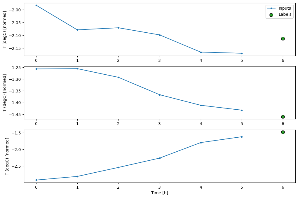
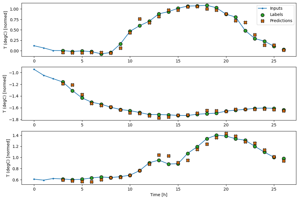
โดยการวางแผนการคาดการณ์ของโมเดลพื้นฐาน สังเกตว่าเป็นเพียงป้ายกำกับที่เลื่อนไปทางขวาภายในหนึ่งชั่วโมง:

wide_window.plot(baseline)

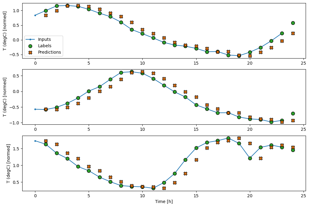
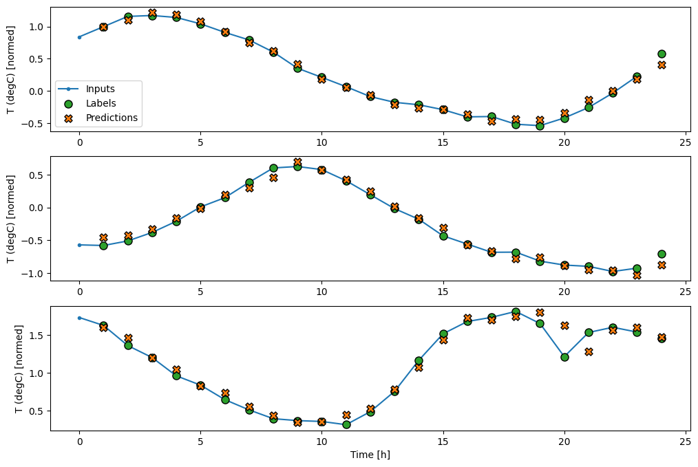
ในแผนภาพสามตัวอย่างข้างต้น โมเดลขั้นตอนเดียวจะดำเนินการตลอด 24 ชั่วโมง สิ่งนี้สมควรได้รับคำอธิบาย:

• เส้น Inputs สีน้ำเงินแสดงอุณหภูมิอินพุตในแต่ละขั้นตอนของเวลา ตัวแบบได้รับคุณสมบัติทั้งหมด พล็อตนี้แสดงเฉพาะอุณหภูมิ
• จุด Labels สีเขียวแสดงค่าการทำนายเป้าหมาย จุดเหล่านี้จะแสดงในเวลาคาดการณ์ ไม่ใช่เวลาอินพุต นั่นคือเหตุผลที่ช่วงของป้ายกำกับเปลี่ยนไป 1 ขั้นตอนเมื่อเทียบกับอินพุต
• การตัดขวางการ Predictions สีส้มเป็นการคาดคะเนของแบบจำลองสำหรับขั้นตอนเวลาการส่งออกแต่ละขั้น หากตัวแบบทำนายได้อย่างสมบูรณ์ การคาดคะเนก็จะตกอยู่ที่ Labels โดยตรง

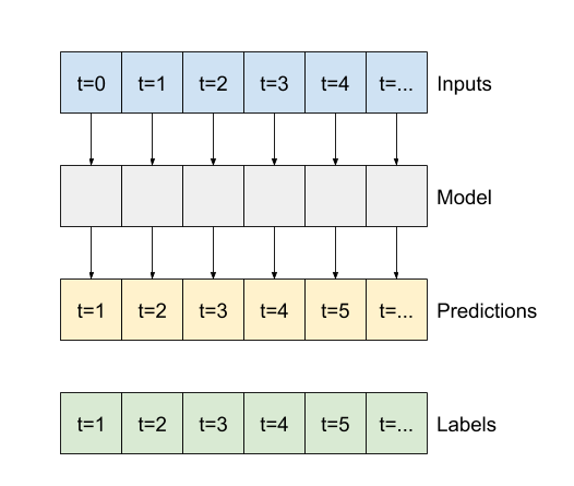
แบบจำลองเชิงเส้น

โมเดล ที่ฝึกได้ที่ง่ายที่สุดที่คุณสามารถใช้กับงานนี้ได้คือการแทรกการแปลงเชิงเส้นระหว่างอินพุตและเอาต์พุต ในกรณีนี้ ผลลัพธ์จากขั้นตอนเวลาจะขึ้นอยู่กับขั้นตอนนั้นเท่านั้น:

เลเยอร์ tf.keras.layers.Dense ที่ไม่มีชุด activation เป็นโมเดลเชิงเส้น เลเยอร์จะเปลี่ยนเฉพาะแกนสุดท้ายของข้อมูลจาก (batch, time, inputs) เป็น (batch, time, units) ; มันถูกนำไปใช้อย่างอิสระกับทุกรายการใน batch งานและแกน time

linear = tf.keras.Sequential([
    tf.keras.layers.Dense(units=1)
])

print('Input shape:', single_step_window.example[0].shape)
print('Output shape:', linear(single_step_window.example[0]).shape)

Input shape: (32, 1, 19)
Output shape: (32, 1, 1)

บทช่วยสอนนี้ฝึกโมเดลต่างๆ มากมาย ดังนั้นให้รวมขั้นตอนการฝึกอบรมเป็นฟังก์ชัน:

MAX_EPOCHS = 20

def compile_and_fit(model, window, patience=2):
  early_stopping = tf.keras.callbacks.EarlyStopping(monitor='val_loss',
                                                    patience=patience,
                                                    mode='min')

  model.compile(loss=tf.losses.MeanSquaredError(),
                optimizer=tf.optimizers.Adam(),
                metrics=[tf.metrics.MeanAbsoluteError()])

  history = model.fit(window.train, epochs=MAX_EPOCHS,
                      validation_data=window.val,
                      callbacks=[early_stopping])
  return history

ฝึกโมเดลและประเมินประสิทธิภาพ:

history = compile_and_fit(linear, single_step_window)

val_performance['Linear'] = linear.evaluate(single_step_window.val)
performance['Linear'] = linear.evaluate(single_step_window.test, verbose=0)

Epoch 1/20
1534/1534 [==============================] - 5s 3ms/step - loss: 0.0586 - mean_absolute_error: 0.1659 - val_loss: 0.0135 - val_mean_absolute_error: 0.0858
Epoch 2/20
1534/1534 [==============================] - 5s 3ms/step - loss: 0.0109 - mean_absolute_error: 0.0772 - val_loss: 0.0093 - val_mean_absolute_error: 0.0711
Epoch 3/20
1534/1534 [==============================] - 5s 3ms/step - loss: 0.0092 - mean_absolute_error: 0.0704 - val_loss: 0.0088 - val_mean_absolute_error: 0.0690
Epoch 4/20
1534/1534 [==============================] - 5s 3ms/step - loss: 0.0091 - mean_absolute_error: 0.0697 - val_loss: 0.0089 - val_mean_absolute_error: 0.0692
Epoch 5/20
1534/1534 [==============================] - 5s 3ms/step - loss: 0.0091 - mean_absolute_error: 0.0697 - val_loss: 0.0088 - val_mean_absolute_error: 0.0685
Epoch 6/20
1534/1534 [==============================] - 5s 3ms/step - loss: 0.0091 - mean_absolute_error: 0.0697 - val_loss: 0.0087 - val_mean_absolute_error: 0.0687
Epoch 7/20
1534/1534 [==============================] - 5s 3ms/step - loss: 0.0091 - mean_absolute_error: 0.0698 - val_loss: 0.0087 - val_mean_absolute_error: 0.0680
Epoch 8/20
1534/1534 [==============================] - 5s 3ms/step - loss: 0.0090 - mean_absolute_error: 0.0695 - val_loss: 0.0087 - val_mean_absolute_error: 0.0683
Epoch 9/20
1534/1534 [==============================] - 5s 3ms/step - loss: 0.0091 - mean_absolute_error: 0.0696 - val_loss: 0.0087 - val_mean_absolute_error: 0.0684
439/439 [==============================] - 1s 2ms/step - loss: 0.0087 - mean_absolute_error: 0.0684

เช่นเดียวกับโมเดล baseline สามารถเรียกใช้โมเดลเชิงเส้นบนแบทช์ของหน้าต่างกว้างได้ ใช้วิธีนี้ โมเดลสร้างชุดการคาดการณ์อิสระตามขั้นตอนเวลาต่อเนื่องกัน แกน time ทำหน้าที่เหมือนแกน batch งานอื่น ไม่มีการโต้ตอบระหว่างการคาดการณ์ในแต่ละขั้นตอนของเวลา

print('Input shape:', wide_window.example[0].shape)
print('Output shape:', baseline(wide_window.example[0]).shape)

Input shape: (32, 24, 19)
Output shape: (32, 24, 1)

ตัวยึดตำแหน่ง60

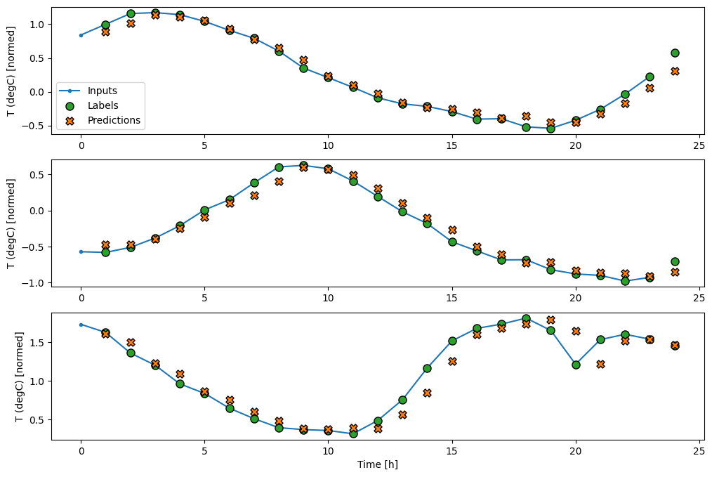
นี่คือพล็อตของตัวอย่างการทำนายบน wide_window สังเกตว่าในหลาย ๆ กรณีการทำนายนั้นดีกว่าการคืนค่าอุณหภูมิอินพุตอย่างชัดเจน แต่ในบางกรณีก็แย่กว่านั้น:

wide_window.plot(linear)

ข้อดีอย่างหนึ่งของตัวแบบเชิงเส้นตรงคือสามารถตีความได้ง่าย คุณสามารถดึงน้ำหนักของเลเยอร์ออกมาและเห็นภาพน้ำหนักที่กำหนดให้กับอินพุตแต่ละรายการ:

plt.bar(x = range(len(train_df.columns)),
        height=linear.layers[0].kernel[:,0].numpy())
axis = plt.gca()
axis.set_xticks(range(len(train_df.columns)))
_ = axis.set_xticklabels(train_df.columns, rotation=90)

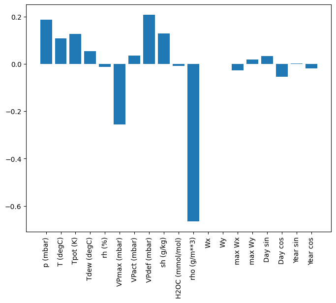
บางครั้งโมเดลไม่ได้วางน้ำหนักมากที่สุดบนอินพุต T (degC) นี่เป็นหนึ่งในความเสี่ยงของการเริ่มต้นแบบสุ่ม

หนาแน่น

ก่อนที่จะใช้แบบจำลองที่ทำงานจริงในขั้นตอนหลายขั้นตอน ควรตรวจสอบประสิทธิภาพของแบบจำลองขั้นตอนอินพุตเดียวที่ลึกกว่า ทรงพลังกว่า

นี่คือโมเดลที่คล้ายกับโมเดล linear ยกเว้นว่าจะซ้อนเลเยอร์ Dense หลายชั้นระหว่างอินพุตและเอาต์พุต:

dense = tf.keras.Sequential([
    tf.keras.layers.Dense(units=64, activation='relu'),
    tf.keras.layers.Dense(units=64, activation='relu'),
    tf.keras.layers.Dense(units=1)
])

history = compile_and_fit(dense, single_step_window)

val_performance['Dense'] = dense.evaluate(single_step_window.val)
performance['Dense'] = dense.evaluate(single_step_window.test, verbose=0)

Epoch 1/20
1534/1534 [==============================] - 7s 4ms/step - loss: 0.0132 - mean_absolute_error: 0.0779 - val_loss: 0.0081 - val_mean_absolute_error: 0.0666
Epoch 2/20
1534/1534 [==============================] - 6s 4ms/step - loss: 0.0081 - mean_absolute_error: 0.0652 - val_loss: 0.0073 - val_mean_absolute_error: 0.0610
Epoch 3/20
1534/1534 [==============================] - 6s 4ms/step - loss: 0.0076 - mean_absolute_error: 0.0627 - val_loss: 0.0072 - val_mean_absolute_error: 0.0618
Epoch 4/20
1534/1534 [==============================] - 6s 4ms/step - loss: 0.0072 - mean_absolute_error: 0.0609 - val_loss: 0.0068 - val_mean_absolute_error: 0.0582
Epoch 5/20
1534/1534 [==============================] - 6s 4ms/step - loss: 0.0072 - mean_absolute_error: 0.0606 - val_loss: 0.0066 - val_mean_absolute_error: 0.0581
Epoch 6/20
1534/1534 [==============================] - 6s 4ms/step - loss: 0.0070 - mean_absolute_error: 0.0594 - val_loss: 0.0067 - val_mean_absolute_error: 0.0579
Epoch 7/20
1534/1534 [==============================] - 6s 4ms/step - loss: 0.0069 - mean_absolute_error: 0.0590 - val_loss: 0.0068 - val_mean_absolute_error: 0.0580
439/439 [==============================] - 1s 3ms/step - loss: 0.0068 - mean_absolute_error: 0.0580

หนาแน่นหลายขั้นตอน

โมเดลขั้นตอนเดียวไม่มีบริบทสำหรับค่าปัจจุบันของอินพุต จะไม่เห็นว่าคุณลักษณะการป้อนข้อมูลเปลี่ยนแปลงไปอย่างไรเมื่อเวลาผ่านไป เพื่อแก้ไขปัญหานี้ โมเดลจำเป็นต้องเข้าถึงขั้นตอนหลายขั้นตอนเมื่อทำการคาดคะเน:

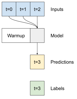
โมเดล baseline linear และ dense จัดการแต่ละขั้นตอนอย่างอิสระ ที่นี่โมเดลจะใช้เวลาหลายขั้นตอนเป็นอินพุตเพื่อสร้างเอาต์พุตเดียว

สร้าง WindowGenerator ที่จะสร้างชุดของอินพุตสามชั่วโมงและฉลากหนึ่งชั่วโมง:

โปรดทราบว่าพารามิเตอร์ shift ของ Window จะสัมพันธ์กับส่วนท้ายของหน้าต่างทั้งสอง

CONV_WIDTH = 3
conv_window = WindowGenerator(
    input_width=CONV_WIDTH,
    label_width=1,
    shift=1,
    label_columns=['T (degC)'])

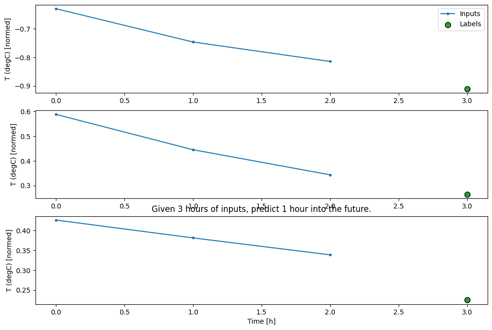
conv_window

Total window size: 4
Input indices: [0 1 2]
Label indices: [3]
Label column name(s): ['T (degC)']

conv_window.plot()
plt.title("Given 3 hours of inputs, predict 1 hour into the future.")

Text(0.5, 1.0, 'Given 3 hours of inputs, predict 1 hour into the future.')

คุณสามารถฝึกโมเดล dense บนหน้าต่างที่มีหลายอินพุตโดยเพิ่ม tf.keras.layers.Flatten เป็นเลเยอร์แรกของโมเดล:

multi_step_dense = tf.keras.Sequential([
    # Shape: (time, features) => (time*features)
    tf.keras.layers.Flatten(),
    tf.keras.layers.Dense(units=32, activation='relu'),
    tf.keras.layers.Dense(units=32, activation='relu'),
    tf.keras.layers.Dense(units=1),
    # Add back the time dimension.
    # Shape: (outputs) => (1, outputs)
    tf.keras.layers.Reshape([1, -1]),
])

print('Input shape:', conv_window.example[0].shape)
print('Output shape:', multi_step_dense(conv_window.example[0]).shape)

Input shape: (32, 3, 19)
Output shape: (32, 1, 1)

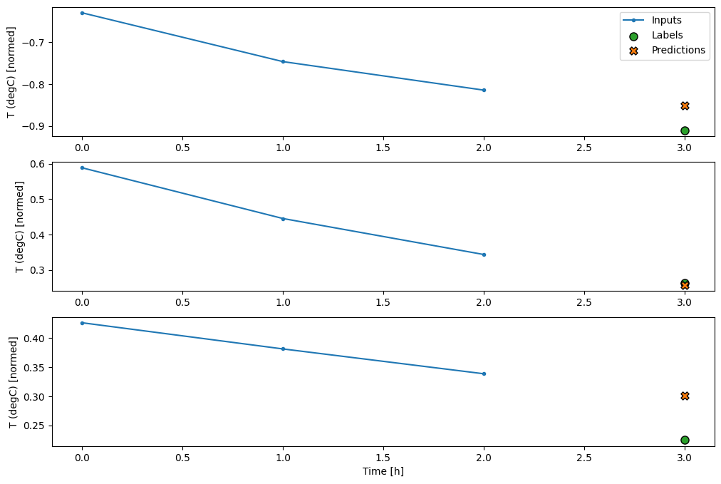
history = compile_and_fit(multi_step_dense, conv_window)

IPython.display.clear_output()
val_performance['Multi step dense'] = multi_step_dense.evaluate(conv_window.val)
performance['Multi step dense'] = multi_step_dense.evaluate(conv_window.test, verbose=0)

438/438 [==============================] - 1s 2ms/step - loss: 0.0070 - mean_absolute_error: 0.0609

conv_window.plot(multi_step_dense)

ข้อเสียเปรียบหลักของแนวทางนี้คือ โมเดลผลลัพธ์สามารถดำเนินการได้บนหน้าต่างอินพุตที่มีรูปร่างนี้เท่านั้น

print('Input shape:', wide_window.example[0].shape)
try:
  print('Output shape:', multi_step_dense(wide_window.example[0]).shape)
except Exception as e:
  print(f'\n{type(e).__name__}:{e}')

Input shape: (32, 24, 19)

ValueError:Exception encountered when calling layer "sequential_2" (type Sequential).

Input 0 of layer "dense_4" is incompatible with the layer: expected axis -1 of input shape to have value 57, but received input with shape (32, 456)

Call arguments received:
  • inputs=tf.Tensor(shape=(32, 24, 19), dtype=float32)
  • training=None
  • mask=None

โมเดลที่โค้งงอได้ในส่วนถัดไปจะแก้ไขปัญหานี้

โครงข่ายประสาทเทียม

เลเยอร์ Convolution ( tf.keras.layers.Conv1D ) ยังใช้เวลาหลายขั้นตอนเป็นอินพุตสำหรับการคาดการณ์แต่ละรายการ

ด้านล่างนี้เป็นรุ่น เดียว กับ multi_step_dense ซึ่งเขียนใหม่ด้วยการบิด

สังเกตการเปลี่ยนแปลง:

• tf.keras.layers.Flatten และ tf.keras.layers.Dense ตัวแรกจะถูกแทนที่ด้วย tf.keras.layers.Conv1D
• tf.keras.layers.Reshape ไม่จำเป็นอีกต่อไป เนื่องจากการบิดจะทำให้แกนเวลาอยู่ในเอาต์พุต

conv_model = tf.keras.Sequential([
    tf.keras.layers.Conv1D(filters=32,
                           kernel_size=(CONV_WIDTH,),
                           activation='relu'),
    tf.keras.layers.Dense(units=32, activation='relu'),
    tf.keras.layers.Dense(units=1),
])

รันบนชุดตัวอย่างเพื่อตรวจสอบว่าโมเดลสร้างเอาต์พุตที่มีรูปร่างที่คาดไว้หรือไม่:

print("Conv model on `conv_window`")
print('Input shape:', conv_window.example[0].shape)
print('Output shape:', conv_model(conv_window.example[0]).shape)

Conv model on `conv_window`
Input shape: (32, 3, 19)
Output shape: (32, 1, 1)

ฝึกและประเมินผลบน conv_window และควรให้ประสิทธิภาพที่คล้ายกับโมเดล multi_step_dense

history = compile_and_fit(conv_model, conv_window)

IPython.display.clear_output()
val_performance['Conv'] = conv_model.evaluate(conv_window.val)
performance['Conv'] = conv_model.evaluate(conv_window.test, verbose=0)

438/438 [==============================] - 1s 3ms/step - loss: 0.0063 - mean_absolute_error: 0.0568

ความแตกต่างระหว่าง conv_model นี้และโมเดล multi_step_dense คือ conv_model สามารถรันบนอินพุตที่มีความยาวเท่าใดก็ได้ เลเยอร์ convolutional ถูกนำไปใช้กับหน้าต่างบานเลื่อนของอินพุต:

หากคุณรันด้วยอินพุตที่กว้างขึ้น มันจะให้เอาต์พุตที่กว้างขึ้น:

print("Wide window")
print('Input shape:', wide_window.example[0].shape)
print('Labels shape:', wide_window.example[1].shape)
print('Output shape:', conv_model(wide_window.example[0]).shape)

Wide window
Input shape: (32, 24, 19)
Labels shape: (32, 24, 1)
Output shape: (32, 22, 1)

โปรดทราบว่าเอาต์พุตสั้นกว่าอินพุต ในการทำให้การฝึกอบรมหรือการวางแผนงาน คุณต้องมีป้ายกำกับและการคาดคะเนให้มีความยาวเท่ากัน ดังนั้นให้สร้าง WindowGenerator เพื่อสร้างหน้าต่างกว้างด้วยขั้นตอนเวลาอินพุตพิเศษสองสามขั้นตอนเพื่อให้ป้ายกำกับและความยาวของการคาดการณ์ตรงกัน:

LABEL_WIDTH = 24
INPUT_WIDTH = LABEL_WIDTH + (CONV_WIDTH - 1)
wide_conv_window = WindowGenerator(
    input_width=INPUT_WIDTH,
    label_width=LABEL_WIDTH,
    shift=1,
    label_columns=['T (degC)'])

wide_conv_window

Total window size: 27
Input indices: [ 0  1  2  3  4  5  6  7  8  9 10 11 12 13 14 15 16 17 18 19 20 21 22 23
 24 25]
Label indices: [ 3  4  5  6  7  8  9 10 11 12 13 14 15 16 17 18 19 20 21 22 23 24 25 26]
Label column name(s): ['T (degC)']

print("Wide conv window")
print('Input shape:', wide_conv_window.example[0].shape)
print('Labels shape:', wide_conv_window.example[1].shape)
print('Output shape:', conv_model(wide_conv_window.example[0]).shape)

Wide conv window
Input shape: (32, 26, 19)
Labels shape: (32, 24, 1)
Output shape: (32, 24, 1)

ตอนนี้คุณสามารถพล็อตการคาดการณ์ของโมเดลในหน้าต่างที่กว้างขึ้น สังเกตขั้นตอนการป้อนข้อมูล 3 ขั้นตอนก่อนการคาดการณ์ครั้งแรก ทุกการคาดการณ์ที่นี่ขึ้นอยู่กับ 3 ขั้นตอนก่อนหน้า:

wide_conv_window.plot(conv_model)

โครงข่ายประสาทกำเริบ

Recurrent Neural Network (RNN) เป็นเครือข่ายประสาทประเภทหนึ่งที่เหมาะสมกับข้อมูลอนุกรมเวลา RNNs ประมวลผลอนุกรมเวลาทีละขั้นตอน โดยคงสถานะภายในจากเวลาเป็นขั้นเป็นตอน

คุณสามารถเรียนรู้เพิ่มเติมในการ สร้างข้อความด้วยบทช่วยสอน RNN และ Recurrent Neural Networks (RNN) พร้อมคู่มือ Keras

ในบทช่วยสอนนี้ คุณจะใช้เลเยอร์ RNN ที่เรียกว่า Long Short-Term Memory ( tf.keras.layers.LSTM )

อาร์กิวเมนต์ตัวสร้างที่สำคัญสำหรับเลเยอร์ Keras RNN ทั้งหมด เช่น tf.keras.layers.LSTM คืออาร์กิวเมนต์ return_sequences การตั้งค่านี้สามารถกำหนดค่าเลเยอร์ได้สองวิธี:

1. หาก False ซึ่งเป็นค่าเริ่มต้น เลเยอร์จะคืนค่าเอาต์พุตของขั้นตอนเวลาสุดท้ายเท่านั้น โดยให้เวลาโมเดลในการอุ่นเครื่องสถานะภายในก่อนที่จะทำการทำนายเพียงครั้งเดียว:

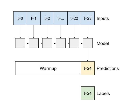
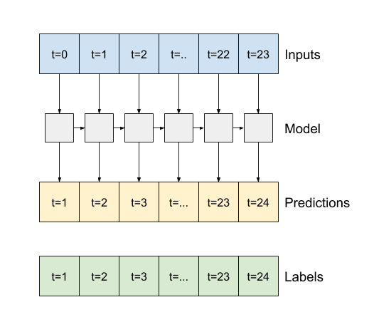
1. หากเป็น True เลเยอร์จะส่งคืนเอาต์พุตสำหรับอินพุตแต่ละรายการ สิ่งนี้มีประโยชน์สำหรับ:
   • การซ้อนเลเยอร์ RNN
   • ฝึกแบบจำลองหลายขั้นตอนพร้อมกัน

lstm_model = tf.keras.models.Sequential([
    # Shape [batch, time, features] => [batch, time, lstm_units]
    tf.keras.layers.LSTM(32, return_sequences=True),
    # Shape => [batch, time, features]
    tf.keras.layers.Dense(units=1)
])

ด้วย return_sequences=True โมเดลสามารถฝึกข้อมูลได้ครั้งละ 24 ชั่วโมง

หมายเหตุ: สิ่งนี้จะให้มุมมองในแง่ร้ายเกี่ยวกับประสิทธิภาพของตัวแบบ ในขั้นตอนแรก โมเดลไม่สามารถเข้าถึงขั้นตอนก่อนหน้า ดังนั้นจึงไม่สามารถทำอะไรได้ดีไปกว่าแบบจำลอง linear และ dense แสดงไว้ก่อนหน้านี้

print('Input shape:', wide_window.example[0].shape)
print('Output shape:', lstm_model(wide_window.example[0]).shape)

Input shape: (32, 24, 19)
Output shape: (32, 24, 1)

history = compile_and_fit(lstm_model, wide_window)

IPython.display.clear_output()
val_performance['LSTM'] = lstm_model.evaluate(wide_window.val)
performance['LSTM'] = lstm_model.evaluate(wide_window.test, verbose=0)

438/438 [==============================] - 1s 3ms/step - loss: 0.0055 - mean_absolute_error: 0.0509

wide_window.plot(lstm_model)

ประสิทธิภาพ

ด้วยชุดข้อมูลนี้ โดยทั่วไปแล้วแต่ละโมเดลจะทำงานได้ดีกว่ารุ่นก่อนหน้าเล็กน้อย:

x = np.arange(len(performance))
width = 0.3
metric_name = 'mean_absolute_error'
metric_index = lstm_model.metrics_names.index('mean_absolute_error')
val_mae = [v[metric_index] for v in val_performance.values()]
test_mae = [v[metric_index] for v in performance.values()]

plt.ylabel('mean_absolute_error [T (degC), normalized]')
plt.bar(x - 0.17, val_mae, width, label='Validation')
plt.bar(x + 0.17, test_mae, width, label='Test')
plt.xticks(ticks=x, labels=performance.keys(),
           rotation=45)
_ = plt.legend()

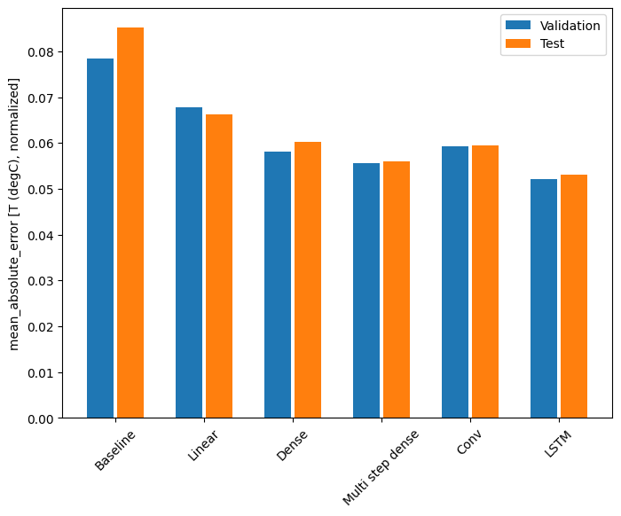
for name, value in performance.items():
  print(f'{name:12s}: {value[1]:0.4f}')

Baseline    : 0.0852
Linear      : 0.0666
Dense       : 0.0573
Multi step dense: 0.0586
Conv        : 0.0577
LSTM        : 0.0518

โมเดลหลายเอาต์พุต

จนถึงตอนนี้ โมเดลทั้งหมดคาดการณ์คุณลักษณะเอาต์พุตเดียว T (degC) สำหรับขั้นตอนเดียว

โมเดลทั้งหมดเหล่านี้สามารถแปลงเพื่อทำนายคุณสมบัติหลาย ๆ อย่างเพียงแค่เปลี่ยนจำนวนหน่วยในเลเยอร์เอาต์พุตและปรับหน้าต่างการฝึกอบรมเพื่อรวมคุณสมบัติทั้งหมดใน labels ( example_labels ):

single_step_window = WindowGenerator(
    # `WindowGenerator` returns all features as labels if you 
    # don't set the `label_columns` argument.
    input_width=1, label_width=1, shift=1)

wide_window = WindowGenerator(
    input_width=24, label_width=24, shift=1)

for example_inputs, example_labels in wide_window.train.take(1):
  print(f'Inputs shape (batch, time, features): {example_inputs.shape}')
  print(f'Labels shape (batch, time, features): {example_labels.shape}')

Inputs shape (batch, time, features): (32, 24, 19)
Labels shape (batch, time, features): (32, 24, 19)

สังเกตว่าแกน features ของป้ายกำกับในขณะนี้มีความลึกเท่ากันกับอินพุต แทนที่จะเป็น 1

พื้นฐาน

สามารถใช้โมเดลพื้นฐานเดียวกัน ( Baseline ) ได้ที่นี่ แต่คราวนี้ใช้คุณลักษณะทั้งหมดซ้ำแทนที่จะเลือก label_index เฉพาะ:

baseline = Baseline()
baseline.compile(loss=tf.losses.MeanSquaredError(),
                 metrics=[tf.metrics.MeanAbsoluteError()])

val_performance = {}
performance = {}
val_performance['Baseline'] = baseline.evaluate(wide_window.val)
performance['Baseline'] = baseline.evaluate(wide_window.test, verbose=0)

438/438 [==============================] - 1s 2ms/step - loss: 0.0886 - mean_absolute_error: 0.1589

หนาแน่น

dense = tf.keras.Sequential([
    tf.keras.layers.Dense(units=64, activation='relu'),
    tf.keras.layers.Dense(units=64, activation='relu'),
    tf.keras.layers.Dense(units=num_features)
])

history = compile_and_fit(dense, single_step_window)

IPython.display.clear_output()
val_performance['Dense'] = dense.evaluate(single_step_window.val)
performance['Dense'] = dense.evaluate(single_step_window.test, verbose=0)

439/439 [==============================] - 1s 3ms/step - loss: 0.0687 - mean_absolute_error: 0.1302

RNN

%%time
wide_window = WindowGenerator(
    input_width=24, label_width=24, shift=1)

lstm_model = tf.keras.models.Sequential([
    # Shape [batch, time, features] => [batch, time, lstm_units]
    tf.keras.layers.LSTM(32, return_sequences=True),
    # Shape => [batch, time, features]
    tf.keras.layers.Dense(units=num_features)
])

history = compile_and_fit(lstm_model, wide_window)

IPython.display.clear_output()
val_performance['LSTM'] = lstm_model.evaluate( wide_window.val)
performance['LSTM'] = lstm_model.evaluate( wide_window.test, verbose=0)

print()

438/438 [==============================] - 1s 3ms/step - loss: 0.0617 - mean_absolute_error: 0.1205

CPU times: user 5min 14s, sys: 1min 17s, total: 6min 31s
Wall time: 2min 8s

ขั้นสูง: การเชื่อมต่อที่เหลือ

โมเดล Baseline จากรุ่นก่อนหน้าใช้ประโยชน์จากข้อเท็จจริงที่ว่าลำดับไม่เปลี่ยนแปลงอย่างมากจากขั้นตอนของเวลาหนึ่งไปอีกขั้นของเวลา แบบจำลองทั้งหมดที่ฝึกในบทช่วยสอนนี้จนถึงขณะนี้ได้รับการสุ่มเริ่มต้น จากนั้นก็ต้องเรียนรู้ว่าผลลัพธ์เป็นการเปลี่ยนแปลงเล็กน้อยจากขั้นตอนเวลาก่อนหน้า

แม้ว่าคุณจะสามารถแก้ไขปัญหานี้ได้ด้วยการเริ่มต้นอย่างระมัดระวัง แต่การสร้างสิ่งนี้ลงในโครงสร้างโมเดลจะง่ายกว่า

เป็นเรื่องปกติในการวิเคราะห์อนุกรมเวลาเพื่อสร้างแบบจำลองที่แทนที่จะคาดการณ์ค่าถัดไป ให้คาดการณ์ว่าค่าจะเปลี่ยนแปลงอย่างไรในขั้นตอนต่อไป ในทำนองเดียวกัน เครือข่ายที่เหลือ —หรือ ResNets— ในการเรียนรู้เชิงลึกหมายถึงสถาปัตยกรรมที่แต่ละเลเยอร์เพิ่มให้กับผลลัพธ์ที่สะสมของแบบจำลอง

นั่นคือวิธีที่คุณใช้ประโยชน์จากความรู้ที่ว่าการเปลี่ยนแปลงควรมีเพียงเล็กน้อย

โดยพื้นฐานแล้ว สิ่งนี้จะเริ่มต้นโมเดลเพื่อให้ตรงกับ Baseline สำหรับงานนี้ จะช่วยให้โมเดลมาบรรจบกันเร็วขึ้น โดยมีประสิทธิภาพที่ดีขึ้นเล็กน้อย

แนวทางนี้สามารถใช้ร่วมกับรูปแบบต่างๆ ที่กล่าวถึงในบทช่วยสอนนี้

ในที่นี้ กำลังนำไปใช้กับโมเดล LSTM โปรดสังเกตการใช้ tf.initializers.zeros เพื่อให้แน่ใจว่าการเปลี่ยนแปลงที่คาดคะเนในเบื้องต้นมีขนาดเล็ก และไม่ทำลายการเชื่อมต่อที่เหลือ ไม่มีปัญหาเรื่องความสมมาตรสำหรับการไล่ระดับสีที่นี่ เนื่องจาก zeros จะใช้เฉพาะในเลเยอร์สุดท้ายเท่านั้น

class ResidualWrapper(tf.keras.Model):
  def __init__(self, model):
    super().__init__()
    self.model = model

  def call(self, inputs, *args, **kwargs):
    delta = self.model(inputs, *args, **kwargs)

    # The prediction for each time step is the input
    # from the previous time step plus the delta
    # calculated by the model.
    return inputs + delta

%%time
residual_lstm = ResidualWrapper(
    tf.keras.Sequential([
    tf.keras.layers.LSTM(32, return_sequences=True),
    tf.keras.layers.Dense(
        num_features,
        # The predicted deltas should start small.
        # Therefore, initialize the output layer with zeros.
        kernel_initializer=tf.initializers.zeros())
]))

history = compile_and_fit(residual_lstm, wide_window)

IPython.display.clear_output()
val_performance['Residual LSTM'] = residual_lstm.evaluate(wide_window.val)
performance['Residual LSTM'] = residual_lstm.evaluate(wide_window.test, verbose=0)
print()

438/438 [==============================] - 1s 3ms/step - loss: 0.0620 - mean_absolute_error: 0.1179

CPU times: user 1min 43s, sys: 26.1 s, total: 2min 9s
Wall time: 43.1 s

ประสิทธิภาพ

นี่คือประสิทธิภาพโดยรวมสำหรับรุ่นที่มีหลายเอาต์พุตเหล่านี้

x = np.arange(len(performance))
width = 0.3

metric_name = 'mean_absolute_error'
metric_index = lstm_model.metrics_names.index('mean_absolute_error')
val_mae = [v[metric_index] for v in val_performance.values()]
test_mae = [v[metric_index] for v in performance.values()]

plt.bar(x - 0.17, val_mae, width, label='Validation')
plt.bar(x + 0.17, test_mae, width, label='Test')
plt.xticks(ticks=x, labels=performance.keys(),
           rotation=45)
plt.ylabel('MAE (average over all outputs)')
_ = plt.legend()

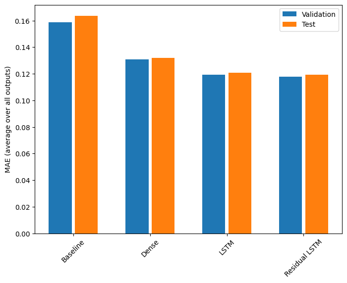
for name, value in performance.items():
  print(f'{name:15s}: {value[1]:0.4f}')

Baseline       : 0.1638
Dense          : 0.1311
LSTM           : 0.1214
Residual LSTM  : 0.1194

ตัวยึดตำแหน่ง113

การแสดงข้างต้นเป็นค่าเฉลี่ยในเอาท์พุตทุกรุ่น

โมเดลหลายขั้นตอน

ทั้งโมเดลเอาต์พุตเดี่ยวและเอาต์พุตหลายรายการในส่วนก่อนหน้าได้ คาดการณ์ขั้นตอนในครั้งเดียว หนึ่งชั่วโมงข้างหน้า

ส่วนนี้จะกล่าวถึงวิธีการขยายโมเดลเหล่านี้เพื่อ คาดการณ์ขั้นตอนหลายขั้นตอน

ในการทำนายแบบหลายขั้นตอน โมเดลจำเป็นต้องเรียนรู้การทำนายช่วงของค่าในอนาคต ดังนั้น จึงไม่เหมือนกับแบบจำลองขั้นตอนเดียวที่มีการทำนายจุดในอนาคตเพียงจุดเดียว โมเดลหลายขั้นตอนจะทำนายลำดับของค่าในอนาคต

มีสองแนวทางคร่าวๆ สำหรับสิ่งนี้:

1. การคาดคะเนนัดเดียวโดยคาดการณ์อนุกรมเวลาทั้งหมดพร้อมกัน
2. การคาดคะเนแบบถดถอยอัตโนมัติโดยที่โมเดลคาดการณ์ขั้นตอนเดียวเท่านั้นและเอาต์พุตของมันถูกป้อนกลับเป็นอินพุต

ในส่วนนี้ แบบจำลองทั้งหมดจะคาดการณ์ คุณลักษณะทั้งหมดในทุกขั้นตอนของเวลาส่งออก

สำหรับแบบจำลองหลายขั้นตอน ข้อมูลการฝึกอีกครั้งจะประกอบด้วยตัวอย่างรายชั่วโมง อย่างไรก็ตาม ในที่นี้ ตัวแบบจะเรียนรู้ที่จะทำนายอนาคต 24 ชั่วโมงจาก 24 ชั่วโมงที่ผ่านมา

นี่คือวัตถุ Window ที่สร้างสไลซ์เหล่านี้จากชุดข้อมูล:

OUT_STEPS = 24
multi_window = WindowGenerator(input_width=24,
                               label_width=OUT_STEPS,
                               shift=OUT_STEPS)

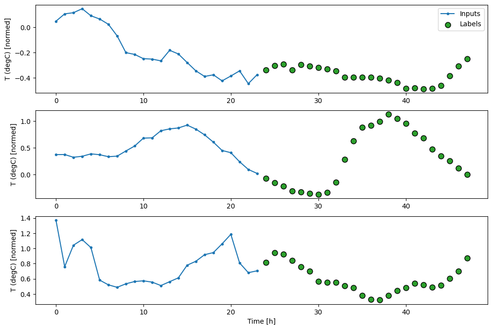
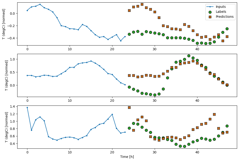
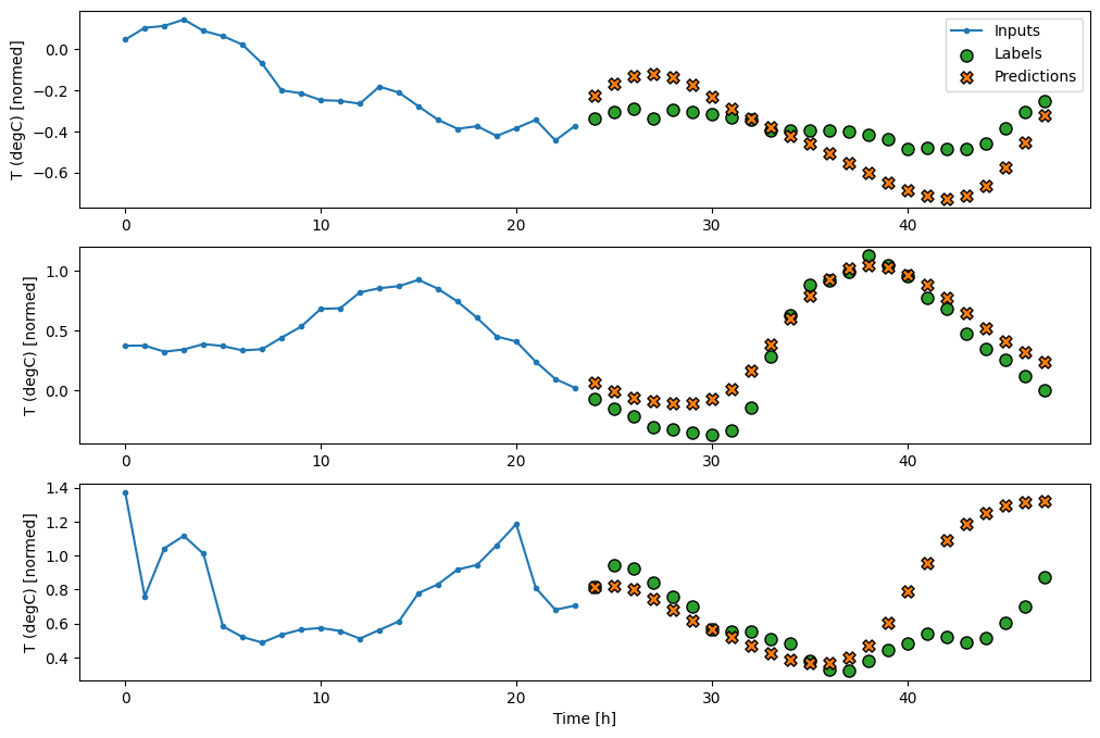
multi_window.plot()
multi_window

Total window size: 48
Input indices: [ 0  1  2  3  4  5  6  7  8  9 10 11 12 13 14 15 16 17 18 19 20 21 22 23]
Label indices: [24 25 26 27 28 29 30 31 32 33 34 35 36 37 38 39 40 41 42 43 44 45 46 47]
Label column name(s): None

ตัวยึดตำแหน่ง115

พื้นฐาน

พื้นฐานง่ายๆ สำหรับงานนี้คือ ทำซ้ำขั้นตอนเวลาป้อนสุดท้ายสำหรับจำนวนขั้นตอนเวลาเอาท์พุตที่ต้องการ:

class MultiStepLastBaseline(tf.keras.Model):
  def call(self, inputs):
    return tf.tile(inputs[:, -1:, :], [1, OUT_STEPS, 1])

last_baseline = MultiStepLastBaseline()
last_baseline.compile(loss=tf.losses.MeanSquaredError(),
                      metrics=[tf.metrics.MeanAbsoluteError()])

multi_val_performance = {}
multi_performance = {}

multi_val_performance['Last'] = last_baseline.evaluate(multi_window.val)
multi_performance['Last'] = last_baseline.evaluate(multi_window.test, verbose=0)
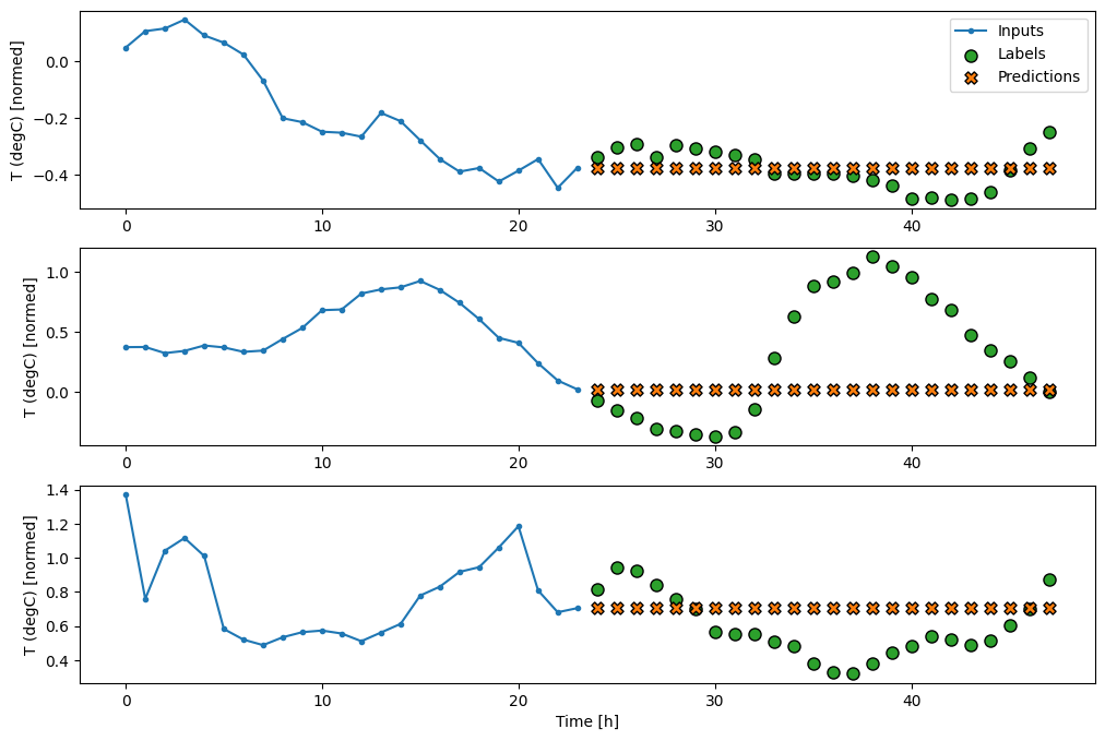
multi_window.plot(last_baseline)

437/437 [==============================] - 1s 2ms/step - loss: 0.6285 - mean_absolute_error: 0.5007

ตัวยึดตำแหน่ง117

เนื่องจากภารกิจนี้คือการคาดการณ์ 24 ชั่วโมงในอนาคต เมื่อให้เวลา 24 ชั่วโมงที่ผ่านมา วิธีง่ายๆ อีกวิธีหนึ่งคือการทำซ้ำของวันก่อนหน้า สมมติว่าพรุ่งนี้จะคล้ายกัน:

class RepeatBaseline(tf.keras.Model):
  def call(self, inputs):
    return inputs

repeat_baseline = RepeatBaseline()
repeat_baseline.compile(loss=tf.losses.MeanSquaredError(),
                        metrics=[tf.metrics.MeanAbsoluteError()])

multi_val_performance['Repeat'] = repeat_baseline.evaluate(multi_window.val)
multi_performance['Repeat'] = repeat_baseline.evaluate(multi_window.test, verbose=0)
multi_window.plot(repeat_baseline)

437/437 [==============================] - 1s 2ms/step - loss: 0.4270 - mean_absolute_error: 0.3959

ตัวยึดตำแหน่ง119

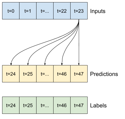
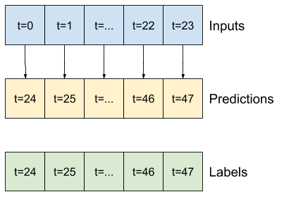
รุ่นยิงครั้งเดียว

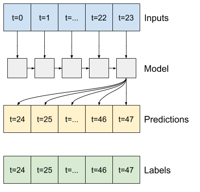
แนวทางระดับสูงวิธีหนึ่งในการแก้ไขปัญหานี้คือการใช้โมเดล "ช็อตเดียว" โดยที่โมเดลจะคาดการณ์ลำดับทั้งหมดในขั้นตอนเดียว

สิ่งนี้สามารถนำไปใช้อย่างมีประสิทธิภาพในฐานะ tf.keras.layers.Dense ด้วย OUT_STEPS*features หน่วยเอาท์พุต โมเดลเพียงแค่ต้องเปลี่ยนรูปร่างที่ส่งออกเป็นที่ต้องการ (OUTPUT_STEPS, features)

เชิงเส้น

แบบจำลองเชิงเส้นอย่างง่ายที่อิงตามขั้นตอนเวลาอินพุตสุดท้ายทำได้ดีกว่าเส้นฐานอย่างใดอย่างหนึ่ง แต่มีกำลังต่ำกว่าปกติ โมเดลจำเป็นต้องคาดการณ์ขั้นตอนเวลา OUTPUT_STEPS จากขั้นตอนเวลาอินพุตเดียวที่มีการฉายภาพเชิงเส้น สามารถจับภาพพฤติกรรมบางส่วนในมิติต่ำเท่านั้น ซึ่งน่าจะขึ้นอยู่กับช่วงเวลาของวันและช่วงเวลาของปีเป็นหลัก

multi_linear_model = tf.keras.Sequential([
    # Take the last time-step.
    # Shape [batch, time, features] => [batch, 1, features]
    tf.keras.layers.Lambda(lambda x: x[:, -1:, :]),
    # Shape => [batch, 1, out_steps*features]
    tf.keras.layers.Dense(OUT_STEPS*num_features,
                          kernel_initializer=tf.initializers.zeros()),
    # Shape => [batch, out_steps, features]
    tf.keras.layers.Reshape([OUT_STEPS, num_features])
])

history = compile_and_fit(multi_linear_model, multi_window)

IPython.display.clear_output()
multi_val_performance['Linear'] = multi_linear_model.evaluate(multi_window.val)
multi_performance['Linear'] = multi_linear_model.evaluate(multi_window.test, verbose=0)
multi_window.plot(multi_linear_model)

437/437 [==============================] - 1s 2ms/step - loss: 0.2559 - mean_absolute_error: 0.3053

ตัวยึดตำแหน่ง121

หนาแน่น

การเพิ่ม tf.keras.layers.Dense ระหว่างอินพุตและเอาต์พุตทำให้โมเดลเชิงเส้นมีพลังมากขึ้น แต่ยังคงอิงตามขั้นตอนเวลาอินพุตเดียวเท่านั้น

multi_dense_model = tf.keras.Sequential([
    # Take the last time step.
    # Shape [batch, time, features] => [batch, 1, features]
    tf.keras.layers.Lambda(lambda x: x[:, -1:, :]),
    # Shape => [batch, 1, dense_units]
    tf.keras.layers.Dense(512, activation='relu'),
    # Shape => [batch, out_steps*features]
    tf.keras.layers.Dense(OUT_STEPS*num_features,
                          kernel_initializer=tf.initializers.zeros()),
    # Shape => [batch, out_steps, features]
    tf.keras.layers.Reshape([OUT_STEPS, num_features])
])

history = compile_and_fit(multi_dense_model, multi_window)

IPython.display.clear_output()
multi_val_performance['Dense'] = multi_dense_model.evaluate(multi_window.val)
multi_performance['Dense'] = multi_dense_model.evaluate(multi_window.test, verbose=0)
multi_window.plot(multi_dense_model)

437/437 [==============================] - 1s 3ms/step - loss: 0.2205 - mean_absolute_error: 0.2837

ตัวยึดตำแหน่ง123

CNN

ตัวแบบ convolutional ทำการคาดคะเนตามประวัติความกว้างคงที่ ซึ่งอาจนำไปสู่ประสิทธิภาพที่ดีกว่าแบบจำลองหนาแน่น เนื่องจากสามารถเห็นการเปลี่ยนแปลงของสิ่งต่างๆ เมื่อเวลาผ่านไป:

CONV_WIDTH = 3
multi_conv_model = tf.keras.Sequential([
    # Shape [batch, time, features] => [batch, CONV_WIDTH, features]
    tf.keras.layers.Lambda(lambda x: x[:, -CONV_WIDTH:, :]),
    # Shape => [batch, 1, conv_units]
    tf.keras.layers.Conv1D(256, activation='relu', kernel_size=(CONV_WIDTH)),
    # Shape => [batch, 1,  out_steps*features]
    tf.keras.layers.Dense(OUT_STEPS*num_features,
                          kernel_initializer=tf.initializers.zeros()),
    # Shape => [batch, out_steps, features]
    tf.keras.layers.Reshape([OUT_STEPS, num_features])
])

history = compile_and_fit(multi_conv_model, multi_window)

IPython.display.clear_output()

multi_val_performance['Conv'] = multi_conv_model.evaluate(multi_window.val)
multi_performance['Conv'] = multi_conv_model.evaluate(multi_window.test, verbose=0)
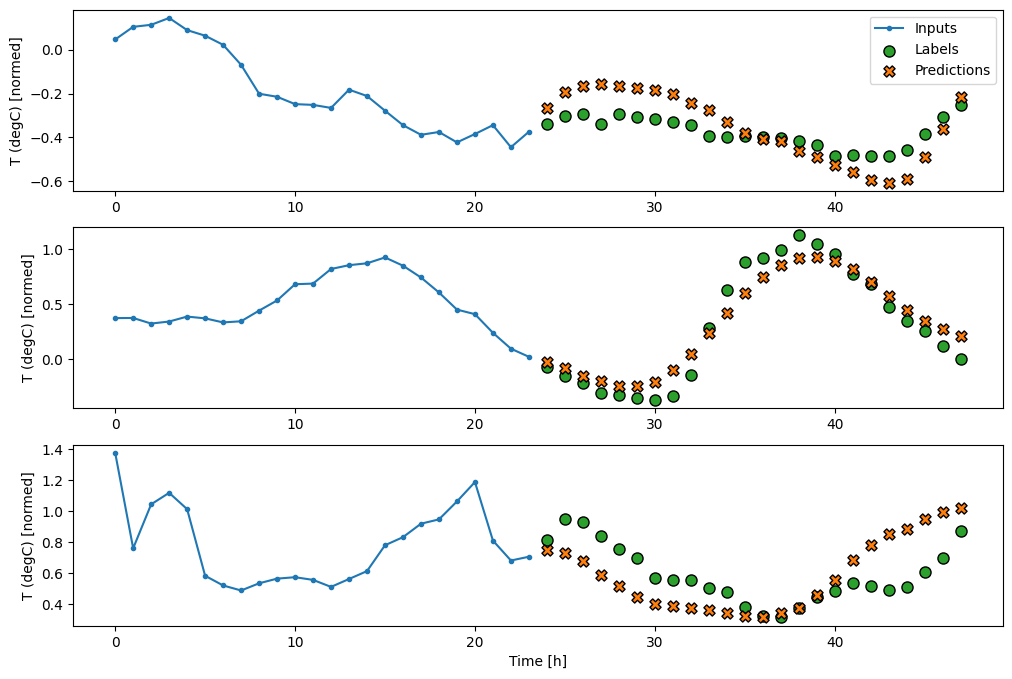
multi_window.plot(multi_conv_model)

437/437 [==============================] - 1s 2ms/step - loss: 0.2158 - mean_absolute_error: 0.2833

ตัวยึดตำแหน่ง125

RNN

โมเดลที่เกิดซ้ำสามารถเรียนรู้การใช้อินพุตที่มีประวัติอันยาวนาน หากเกี่ยวข้องกับการคาดการณ์ที่โมเดลกำลังทำ ที่นี่ โมเดลจะสะสมสถานะภายในเป็นเวลา 24 ชั่วโมง ก่อนทำการทำนายเพียงครั้งเดียวสำหรับ 24 ชั่วโมงข้างหน้า

ในรูปแบบช็อตเดียวนี้ LSTM จำเป็นต้องสร้างเอาต์พุตในขั้นตอนสุดท้ายเท่านั้น ดังนั้นให้ตั้งค่า return_sequences=False ใน tf.keras.layers.LSTM

multi_lstm_model = tf.keras.Sequential([
    # Shape [batch, time, features] => [batch, lstm_units].
    # Adding more `lstm_units` just overfits more quickly.
    tf.keras.layers.LSTM(32, return_sequences=False),
    # Shape => [batch, out_steps*features].
    tf.keras.layers.Dense(OUT_STEPS*num_features,
                          kernel_initializer=tf.initializers.zeros()),
    # Shape => [batch, out_steps, features].
    tf.keras.layers.Reshape([OUT_STEPS, num_features])
])

history = compile_and_fit(multi_lstm_model, multi_window)

IPython.display.clear_output()

multi_val_performance['LSTM'] = multi_lstm_model.evaluate(multi_window.val)
multi_performance['LSTM'] = multi_lstm_model.evaluate(multi_window.test, verbose=0)
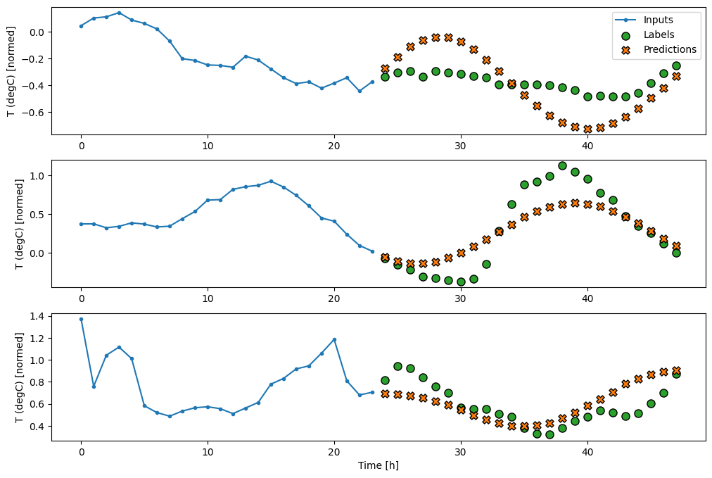
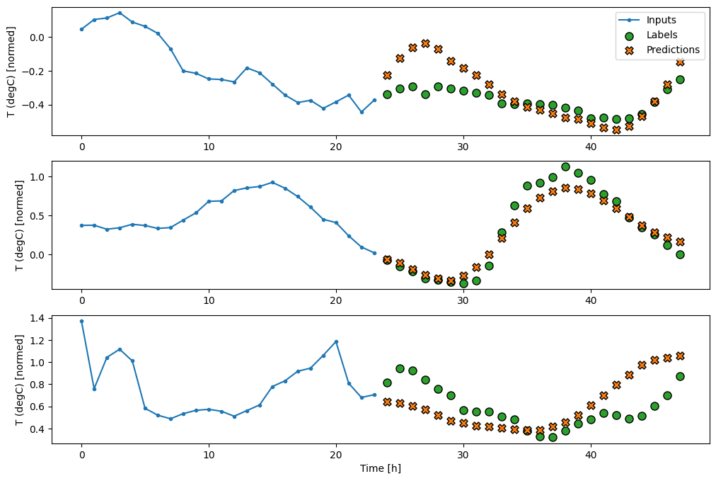
multi_window.plot(multi_lstm_model)

437/437 [==============================] - 1s 3ms/step - loss: 0.2159 - mean_absolute_error: 0.2863

ตัวยึดตำแหน่ง127

ขั้นสูง: โมเดลการถดถอยอัตโนมัติ

โมเดลข้างต้นคาดการณ์ลำดับเอาต์พุตทั้งหมดในขั้นตอนเดียว

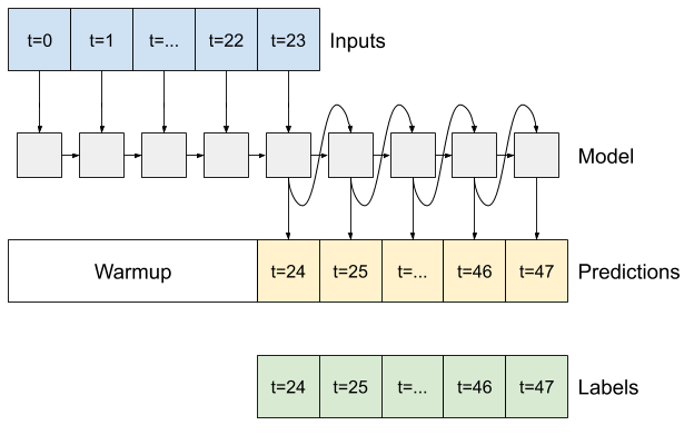
ในบางกรณี อาจเป็นประโยชน์สำหรับตัวแบบในการแยกการคาดคะเนนี้เป็นขั้นตอนเวลาแต่ละขั้น จากนั้น เอาต์พุตของแต่ละโมเดลสามารถป้อนกลับเข้าไปในตัวเองได้ในแต่ละขั้นตอน และการคาดการณ์สามารถทำการปรับเงื่อนไขกับรุ่นก่อนหน้าได้ เช่นเดียวกับใน Generating Sequences With Recurrent Neural Networks แบบคลาสสิก

ข้อดีอย่างหนึ่งที่ชัดเจนของรูปแบบนี้คือสามารถตั้งค่าให้ผลิตผลงานที่มีความยาวต่างกันได้

คุณสามารถใช้โมเดลหลายเอาต์พุตแบบขั้นตอนเดียวที่ได้รับการฝึกฝนในช่วงครึ่งแรกของบทช่วยสอนนี้และเรียกใช้ในลูปป้อนกลับอัตโนมัติ แต่ที่นี่ คุณจะเน้นที่การสร้างแบบจำลองที่ได้รับการฝึกอบรมอย่างชัดเจนให้ทำเช่นนั้น

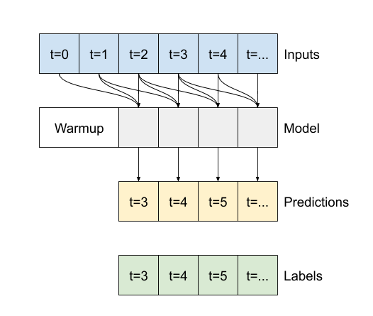
RNN

บทช่วยสอนนี้สร้างเฉพาะแบบจำลอง RNN แบบถดถอยอัตโนมัติ แต่รูปแบบนี้สามารถนำไปใช้กับแบบจำลองใดๆ ที่ออกแบบมาเพื่อแสดงขั้นตอนเวลาเดียว

โมเดลจะมีรูปแบบพื้นฐานเหมือนกับโมเดล LSTM แบบขั้นตอนเดียวจากก่อนหน้านี้: เลเยอร์ tf.keras.layers.LSTM ตามด้วยเลเยอร์ tf.keras.layers.Dense ที่แปลงเอาต์พุตของเลเยอร์ LSTM เป็นการคาดคะเนโมเดล

tf.keras.layers.LSTM คือ tf.keras.layers.LSTMCell ที่อยู่ใน tf.keras.layers.RNN ระดับที่สูงกว่า ซึ่งจัดการสถานะและผลลัพธ์ของลำดับสำหรับคุณ (ตรวจสอบ Recurrent Neural Networks (RNN) กับ Keras คำแนะนำสำหรับรายละเอียด)

ในกรณีนี้ โมเดลต้องจัดการอินพุตด้วยตนเองสำหรับแต่ละขั้นตอน ดังนั้นจึงใช้ tf.keras.layers.LSTMCell โดยตรงสำหรับอินเทอร์เฟซขั้นตอนเดียวระดับล่าง

class FeedBack(tf.keras.Model):
  def __init__(self, units, out_steps):
    super().__init__()
    self.out_steps = out_steps
    self.units = units
    self.lstm_cell = tf.keras.layers.LSTMCell(units)
    # Also wrap the LSTMCell in an RNN to simplify the `warmup` method.
    self.lstm_rnn = tf.keras.layers.RNN(self.lstm_cell, return_state=True)
    self.dense = tf.keras.layers.Dense(num_features)

feedback_model = FeedBack(units=32, out_steps=OUT_STEPS)

วิธีแรกที่โมเดลนี้ต้องการคือวิธีการ warmup เพื่อเริ่มต้นสถานะภายในตามอินพุต เมื่อผ่านการฝึกอบรมแล้ว สถานะนี้จะรวบรวมส่วนที่เกี่ยวข้องของประวัติอินพุต ซึ่งเทียบเท่ากับโมเดล LSTM แบบขั้นตอนเดียวจากรุ่นก่อนหน้า:

def warmup(self, inputs):
  # inputs.shape => (batch, time, features)
  # x.shape => (batch, lstm_units)
  x, *state = self.lstm_rnn(inputs)

  # predictions.shape => (batch, features)
  prediction = self.dense(x)
  return prediction, state

FeedBack.warmup = warmup

เมธอดนี้ส่งคืนการทำนายขั้นตอนเดียวและสถานะภายในของ LSTM :

prediction, state = feedback_model.warmup(multi_window.example[0])
prediction.shape

TensorShape([32, 19])

ตัวยึดตำแหน่ง132

ด้วยสถานะของ RNN และการคาดคะเนเบื้องต้น ตอนนี้คุณสามารถทำซ้ำแบบจำลองที่ป้อนการคาดคะเนในแต่ละขั้นตอนกลับเป็นอินพุตได้

วิธีที่ง่ายที่สุดในการรวบรวมการคาดการณ์ผลลัพธ์คือการใช้รายการ Python และ tf.stack หลังลูป

หมายเหตุ: การซ้อนรายการ Python แบบนี้ใช้ได้เฉพาะกับการดำเนินการแบบกระตือรือร้น ใช้ Model.compile(..., run_eagerly=True) สำหรับการฝึกอบรม หรือด้วยเอาต์พุตความยาวคงที่ สำหรับความยาวเอาต์พุตแบบไดนามิก คุณจะต้องใช้ tf.TensorArray แทนรายการ Python และใช้ tf.range แทน Python range

def call(self, inputs, training=None):
  # Use a TensorArray to capture dynamically unrolled outputs.
  predictions = []
  # Initialize the LSTM state.
  prediction, state = self.warmup(inputs)

  # Insert the first prediction.
  predictions.append(prediction)

  # Run the rest of the prediction steps.
  for n in range(1, self.out_steps):
    # Use the last prediction as input.
    x = prediction
    # Execute one lstm step.
    x, state = self.lstm_cell(x, states=state,
                              training=training)
    # Convert the lstm output to a prediction.
    prediction = self.dense(x)
    # Add the prediction to the output.
    predictions.append(prediction)

  # predictions.shape => (time, batch, features)
  predictions = tf.stack(predictions)
  # predictions.shape => (batch, time, features)
  predictions = tf.transpose(predictions, [1, 0, 2])
  return predictions

FeedBack.call = call

ทดสอบรันโมเดลนี้กับอินพุตตัวอย่าง:

print('Output shape (batch, time, features): ', feedback_model(multi_window.example[0]).shape)

Output shape (batch, time, features):  (32, 24, 19)

ตัวยึดตำแหน่ง135

ตอนนี้ ฝึกโมเดล:

history = compile_and_fit(feedback_model, multi_window)

IPython.display.clear_output()

multi_val_performance['AR LSTM'] = feedback_model.evaluate(multi_window.val)
multi_performance['AR LSTM'] = feedback_model.evaluate(multi_window.test, verbose=0)
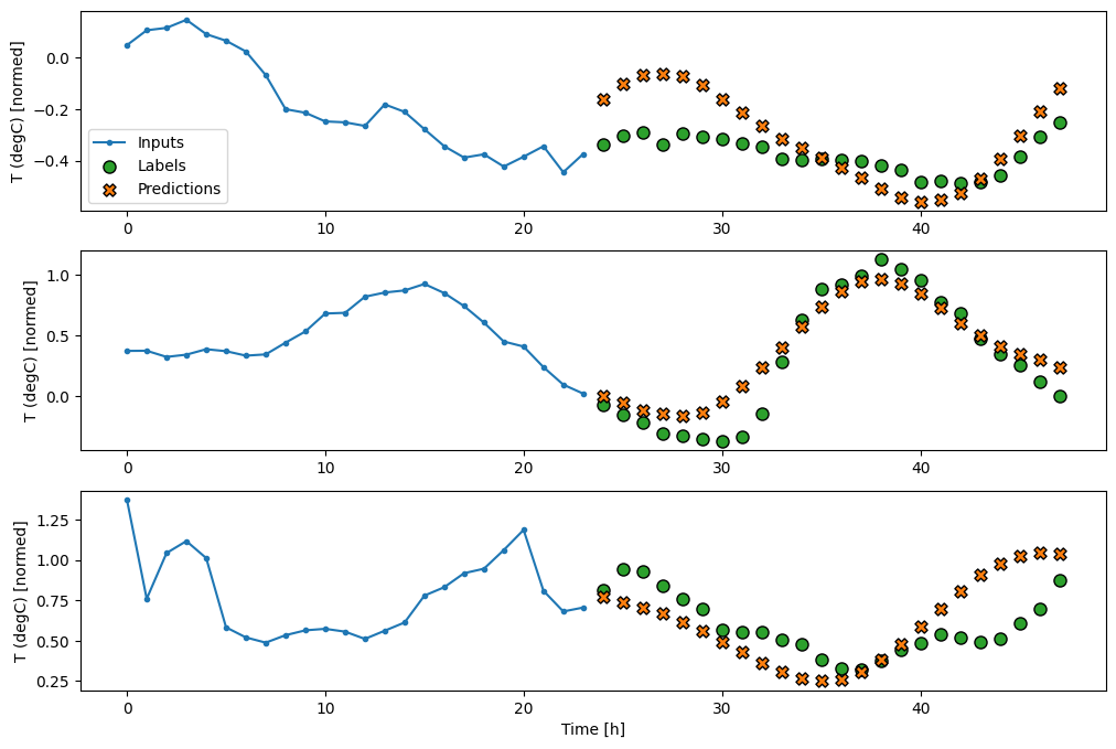
multi_window.plot(feedback_model)

437/437 [==============================] - 3s 8ms/step - loss: 0.2269 - mean_absolute_error: 0.3011

ประสิทธิภาพ

มีผลตอบแทนลดลงอย่างเห็นได้ชัดเนื่องจากความซับซ้อนของแบบจำลองในปัญหานี้:

x = np.arange(len(multi_performance))
width = 0.3

metric_name = 'mean_absolute_error'
metric_index = lstm_model.metrics_names.index('mean_absolute_error')
val_mae = [v[metric_index] for v in multi_val_performance.values()]
test_mae = [v[metric_index] for v in multi_performance.values()]

plt.bar(x - 0.17, val_mae, width, label='Validation')
plt.bar(x + 0.17, test_mae, width, label='Test')
plt.xticks(ticks=x, labels=multi_performance.keys(),
           rotation=45)
plt.ylabel(f'MAE (average over all times and outputs)')
_ = plt.legend()

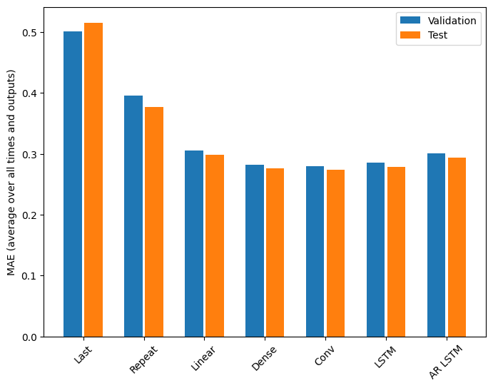
เมตริกสำหรับโมเดลหลายเอาต์พุตในครึ่งแรกของบทช่วยสอนนี้แสดงประสิทธิภาพโดยเฉลี่ยในฟีเจอร์เอาต์พุตทั้งหมด การแสดงเหล่านี้มีความคล้ายคลึงกันแต่ยังเฉลี่ยตามขั้นตอนของเวลาส่งออกด้วย

for name, value in multi_performance.items():
  print(f'{name:8s}: {value[1]:0.4f}')

Last    : 0.5157
Repeat  : 0.3774
Linear  : 0.2977
Dense   : 0.2781
Conv    : 0.2796
LSTM    : 0.2767
AR LSTM : 0.2901

กำไรที่ได้รับจากแบบจำลองหนาแน่นไปเป็นแบบจำลองการบิดเบี้ยวและแบบที่เกิดซ้ำนั้นมีเพียงไม่กี่เปอร์เซ็นต์ (ถ้ามี) และแบบจำลองการถดถอยอัตโนมัติกลับแย่ลงอย่างเห็นได้ชัด ดังนั้นแนวทางที่ซับซ้อนกว่านี้จึงอาจไม่คุ้มค่าในขณะที่แก้ไขปัญหา นี้ แต่ก็ไม่มีทางรู้ได้หากไม่ได้ลอง และแบบจำลองเหล่านี้อาจมีประโยชน์สำหรับปัญหา ของคุณ

ขั้นตอนถัดไป

บทช่วยสอนนี้เป็นการแนะนำสั้นๆ เกี่ยวกับการคาดการณ์อนุกรมเวลาโดยใช้ TensorFlow

หากต้องการเรียนรู้เพิ่มเติม โปรดดูที่:

• บทที่ 15 ของ Hands-on Machine Learning ด้วย Scikit-Learn, Keras และ TensorFlow รุ่นที่ 2
• บทที่ 6 ของ Deep Learning ด้วย Python
• บทที่ 8 ของ บทนำของ Udacity เกี่ยวกับ TensorFlow สำหรับการเรียนรู้เชิงลึก รวมถึง สมุดบันทึกการออกกำลังกาย

นอกจากนี้ โปรดจำไว้ว่าคุณสามารถใช้ โมเดลอนุกรมเวลาแบบคลาสสิก ใน TensorFlow ได้—บทช่วยสอนนี้เน้นที่ฟังก์ชันในตัวของ TensorFlow เท่านั้น