| | |  GitHub पर स्रोत देखें GitHub पर स्रोत देखें | |
संरचनात्मक समय श्रृंखला (एसटीएस) मॉडल के साथ फिटिंग और पूर्वानुमान करते समय यह नोटबुक एक (गैर-गॉसियन) अवलोकन मॉडल को शामिल करने के लिए टीएफपी अनुमानित अनुमान उपकरण के उपयोग को प्रदर्शित करता है। इस उदाहरण में, हम असतत गणना डेटा के साथ काम करने के लिए पॉइसन अवलोकन मॉडल का उपयोग करेंगे।
import time
import matplotlib.pyplot as plt
import numpy as np

import tensorflow.compat.v2 as tf
import tensorflow_probability as tfp

from tensorflow_probability import bijectors as tfb
from tensorflow_probability import distributions as tfd

tf.enable_v2_behavior()
सिंथेटिक डेटा
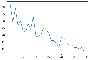
पहले हम कुछ सिंथेटिक गणना डेटा उत्पन्न करेंगे:
num_timesteps = 30
observed_counts = np.round(3 + np.random.lognormal(np.log(np.linspace(
    num_timesteps, 5, num=num_timesteps)), 0.20, size=num_timesteps))
observed_counts = observed_counts.astype(np.float32)
plt.plot(observed_counts)
[<matplotlib.lines.Line2D at 0x7f940ae958d0>]
नमूना
हम बेतरतीब ढंग से चलने वाली रैखिक प्रवृत्ति के साथ एक साधारण मॉडल निर्दिष्ट करेंगे:
def build_model(approximate_unconstrained_rates):
  trend = tfp.sts.LocalLinearTrend(
      observed_time_series=approximate_unconstrained_rates)
  return tfp.sts.Sum([trend],
                     observed_time_series=approximate_unconstrained_rates)
देखे गए समय श्रृंखला पर काम करने के बजाय, यह मॉडल पॉइसन दर पैरामीटर की श्रृंखला पर काम करेगा जो अवलोकनों को नियंत्रित करता है।
चूंकि पॉइसन दरें सकारात्मक होनी चाहिए, इसलिए हम वास्तविक-मूल्यवान एसटीएस मॉडल को सकारात्मक मूल्यों पर वितरण में बदलने के लिए एक बायजेक्टर का उपयोग करेंगे। Softplus परिवर्तन \(y = \log(1 + \exp(x))\) के बाद से यह लगभग सकारात्मक मूल्यों के लिए रेखीय है, एक स्वाभाविक पसंद है, लेकिन इस तरह के रूप में अन्य विकल्पों Exp (जो एक lognormal यादृच्छिक पैदल दूरी में सामान्य यादृच्छिक की पैदल दूरी पर बदल देती है) भी संभव हैं।
positive_bijector = tfb.Softplus()  # Or tfb.Exp()

# Approximate the unconstrained Poisson rate just to set heuristic priors.
# We could avoid this by passing explicit priors on all model params.
approximate_unconstrained_rates = positive_bijector.inverse(
    tf.convert_to_tensor(observed_counts) + 0.01)
sts_model = build_model(approximate_unconstrained_rates)
गैर-गॉसियन अवलोकन मॉडल के लिए अनुमानित अनुमान का उपयोग करने के लिए, हम एसटीएस मॉडल को टीएफपी संयुक्त वितरण के रूप में एन्कोड करेंगे। इस संयुक्त वितरण में यादृच्छिक चर एसटीएस मॉडल के पैरामीटर, गुप्त पॉइसन दरों की समय श्रृंखला, और देखी गई गणनाएं हैं।
def sts_with_poisson_likelihood_model():
  # Encode the parameters of the STS model as random variables.
  param_vals = []
  for param in sts_model.parameters:
    param_val = yield param.prior
    param_vals.append(param_val)

  # Use the STS model to encode the log- (or inverse-softplus)
  # rate of a Poisson.
  unconstrained_rate = yield sts_model.make_state_space_model(
      num_timesteps, param_vals)
  rate = positive_bijector.forward(unconstrained_rate[..., 0])
  observed_counts = yield tfd.Poisson(rate, name='observed_counts')

model = tfd.JointDistributionCoroutineAutoBatched(sts_with_poisson_likelihood_model)
अनुमान की तैयारी
प्रेक्षित गणनाओं को देखते हुए हम मॉडल में प्रेक्षित मात्राओं का अनुमान लगाना चाहते हैं। सबसे पहले, हम प्रेक्षित गणनाओं पर संयुक्त लॉग घनत्व को कंडीशन करते हैं।
pinned_model = model.experimental_pin(observed_counts=observed_counts)
हमें यह सुनिश्चित करने के लिए एक विवश बिजेक्टर की भी आवश्यकता होगी कि अनुमान एसटीएस मॉडल के मापदंडों पर बाधाओं का सम्मान करता है (उदाहरण के लिए, तराजू सकारात्मक होना चाहिए)।
constraining_bijector = pinned_model.experimental_default_event_space_bijector()
एचएमसी के साथ निष्कर्ष
हम एचएमसी (विशेष रूप से, एनयूटीएस) का उपयोग संयुक्त पोस्टीरियर ओवर मॉडल पैरामीटर और गुप्त दरों से नमूना लेने के लिए करेंगे।
यह एचएमसी के साथ एक मानक एसटीएस मॉडल को फिट करने की तुलना में काफी धीमा होगा, क्योंकि मॉडल के (अपेक्षाकृत कम संख्या में) मापदंडों के अलावा हमें पॉइसन दरों की पूरी श्रृंखला का भी अनुमान लगाना होगा। इसलिए हम अपेक्षाकृत कम चरणों के लिए दौड़ेंगे; उन अनुप्रयोगों के लिए जहां अनुमान की गुणवत्ता महत्वपूर्ण है, इन मूल्यों को बढ़ाने या कई श्रृंखलाओं को चलाने के लिए समझ में आ सकता है।
नमूना विन्यास
# Allow external control of sampling to reduce test runtimes.
num_results = 500 # @param { isTemplate: true}
num_results = int(num_results)

num_burnin_steps = 100 # @param { isTemplate: true}
num_burnin_steps = int(num_burnin_steps)
पहले हम एक नमूना निर्दिष्ट करें और फिर उपयोग sample_chain नमूने का उत्पादन करने के लिए है कि नमूना गिरी को चलाने के लिए।
sampler = tfp.mcmc.TransformedTransitionKernel(
    tfp.mcmc.NoUTurnSampler(
        target_log_prob_fn=pinned_model.unnormalized_log_prob,
        step_size=0.1),
    bijector=constraining_bijector)

adaptive_sampler = tfp.mcmc.DualAveragingStepSizeAdaptation(
    inner_kernel=sampler,
    num_adaptation_steps=int(0.8 * num_burnin_steps),
    target_accept_prob=0.75)

initial_state = constraining_bijector.forward(
    type(pinned_model.event_shape)(
        *(tf.random.normal(part_shape)
          for part_shape in constraining_bijector.inverse_event_shape(
              pinned_model.event_shape))))
# Speed up sampling by tracing with `tf.function`.
@tf.function(autograph=False, jit_compile=True)
def do_sampling():
  return tfp.mcmc.sample_chain(
      kernel=adaptive_sampler,
      current_state=initial_state,
      num_results=num_results,
      num_burnin_steps=num_burnin_steps,
      trace_fn=None)

t0 = time.time()
samples = do_sampling()
t1 = time.time()
print("Inference ran in {:.2f}s.".format(t1-t0))
Inference ran in 24.83s.
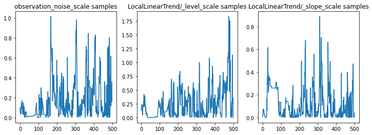
हम पैरामीटर के निशान की जांच करके अनुमान की विवेक-जांच कर सकते हैं। इस मामले में उन्होंने डेटा के लिए कई स्पष्टीकरणों का पता लगाया है, जो अच्छा है, हालांकि अधिक नमूने यह निर्धारित करने में सहायक होंगे कि श्रृंखला कितनी अच्छी तरह मिश्रण कर रही है।
f = plt.figure(figsize=(12, 4))
for i, param in enumerate(sts_model.parameters):
  ax = f.add_subplot(1, len(sts_model.parameters), i + 1)
  ax.plot(samples[i])
  ax.set_title("{} samples".format(param.name))
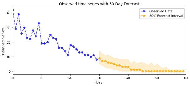
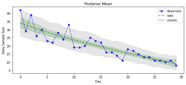
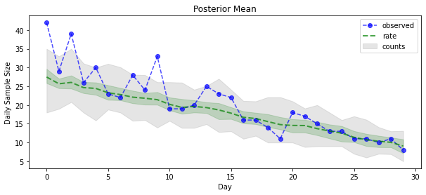
अब अदायगी के लिए: आइए देखते हैं पॉइसन दरों पर पीछे की ओर! हम प्रेक्षित गणनाओं पर 80% भविष्य कहनेवाला अंतराल भी प्लॉट करेंगे, और यह जाँच सकते हैं कि इस अंतराल में लगभग 80% गणनाएँ शामिल हैं जो हमने वास्तव में देखी हैं।
param_samples = samples[:-1]
unconstrained_rate_samples = samples[-1][..., 0]
rate_samples = positive_bijector.forward(unconstrained_rate_samples)

plt.figure(figsize=(10, 4))
mean_lower, mean_upper = np.percentile(rate_samples, [10, 90], axis=0)
pred_lower, pred_upper = np.percentile(np.random.poisson(rate_samples),
                                       [10, 90], axis=0)

_ = plt.plot(observed_counts, color="blue", ls='--', marker='o', label='observed', alpha=0.7)
_ = plt.plot(np.mean(rate_samples, axis=0), label='rate', color="green", ls='dashed', lw=2, alpha=0.7)
_ = plt.fill_between(np.arange(0, 30), mean_lower, mean_upper, color='green', alpha=0.2)
_ = plt.fill_between(np.arange(0, 30), pred_lower, pred_upper, color='grey', label='counts', alpha=0.2)
plt.xlabel("Day")
plt.ylabel("Daily Sample Size")
plt.title("Posterior Mean")
plt.legend()
<matplotlib.legend.Legend at 0x7f93ffd35550>
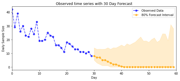
पूर्वानुमान
प्रेक्षित गणनाओं का पूर्वानुमान लगाने के लिए, हम अव्यक्त दरों पर पूर्वानुमान वितरण बनाने के लिए मानक एसटीएस टूल का उपयोग करेंगे (अप्रतिबंधित स्थान में, फिर से चूंकि एसटीएस को वास्तविक-मूल्यवान डेटा मॉडल करने के लिए डिज़ाइन किया गया है), फिर नमूना पूर्वानुमानों को पॉइसन अवलोकन के माध्यम से पास करें नमूना:
def sample_forecasted_counts(sts_model, posterior_latent_rates,
                             posterior_params, num_steps_forecast,
                             num_sampled_forecasts):

  # Forecast the future latent unconstrained rates, given the inferred latent
  # unconstrained rates and parameters.
  unconstrained_rates_forecast_dist = tfp.sts.forecast(sts_model,
    observed_time_series=unconstrained_rate_samples,
    parameter_samples=posterior_params,
    num_steps_forecast=num_steps_forecast)

  # Transform the forecast to positive-valued Poisson rates.
  rates_forecast_dist = tfd.TransformedDistribution(
      unconstrained_rates_forecast_dist,
      positive_bijector)

  # Sample from the forecast model following the chain rule:
  # P(counts) = P(counts | latent_rates)P(latent_rates)
  sampled_latent_rates = rates_forecast_dist.sample(num_sampled_forecasts)
  sampled_forecast_counts = tfd.Poisson(rate=sampled_latent_rates).sample()

  return sampled_forecast_counts, sampled_latent_rates

forecast_samples, rate_samples = sample_forecasted_counts(
   sts_model,
   posterior_latent_rates=unconstrained_rate_samples,
   posterior_params=param_samples,
   # Days to forecast:
   num_steps_forecast=30,
   num_sampled_forecasts=100)
forecast_samples = np.squeeze(forecast_samples)
def plot_forecast_helper(data, forecast_samples, CI=90):
  """Plot the observed time series alongside the forecast."""
  plt.figure(figsize=(10, 4))
  forecast_median = np.median(forecast_samples, axis=0)

  num_steps = len(data)
  num_steps_forecast = forecast_median.shape[-1]

  plt.plot(np.arange(num_steps), data, lw=2, color='blue', linestyle='--', marker='o',
           label='Observed Data', alpha=0.7)

  forecast_steps = np.arange(num_steps, num_steps+num_steps_forecast)

  CI_interval = [(100 - CI)/2, 100 - (100 - CI)/2]
  lower, upper = np.percentile(forecast_samples, CI_interval, axis=0)

  plt.plot(forecast_steps, forecast_median, lw=2, ls='--', marker='o', color='orange',
           label=str(CI) + '% Forecast Interval', alpha=0.7)
  plt.fill_between(forecast_steps,
                   lower,
                   upper, color='orange', alpha=0.2)

  plt.xlim([0, num_steps+num_steps_forecast])
  ymin, ymax = min(np.min(forecast_samples), np.min(data)), max(np.max(forecast_samples), np.max(data))
  yrange = ymax-ymin
  plt.title("{}".format('Observed time series with ' + str(num_steps_forecast) + ' Day Forecast'))
  plt.xlabel('Day')
  plt.ylabel('Daily Sample Size')
  plt.legend()
plot_forecast_helper(observed_counts, forecast_samples, CI=80)
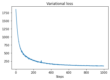
VI अनुमान
परिवर्तन संबंधी अनुमान समस्याग्रस्त जब एक पूर्णकालिक श्रृंखला का निष्कर्ष निकालते, हमारे अनुमानित मायने रखता है की तरह (के रूप में मानक एसटीएस मॉडल में के रूप में, एक समय श्रृंखला का सिर्फ मानकों के खिलाफ) हो सकता है। मानक धारणा है कि चर के स्वतंत्र पोस्टीरियर हैं, काफी गलत है, क्योंकि प्रत्येक टाइमस्टेप अपने पड़ोसियों के साथ सहसंबद्ध है, जिससे अनिश्चितता को कम करके आंका जा सकता है। इस कारण से, एचएमसी पूर्णकालिक श्रृंखला पर अनुमानित अनुमान के लिए एक बेहतर विकल्प हो सकता है। हालांकि, VI काफी तेज हो सकता है, और मॉडल प्रोटोटाइप के लिए उपयोगी हो सकता है या ऐसे मामलों में जहां इसका प्रदर्शन अनुभवजन्य रूप से 'काफी अच्छा' दिखाया जा सकता है।
अपने मॉडल को VI के साथ फिट करने के लिए, हम बस एक सरोगेट पोस्टीरियर का निर्माण और अनुकूलन करते हैं:
surrogate_posterior = tfp.experimental.vi.build_factored_surrogate_posterior(
    event_shape=pinned_model.event_shape,
    bijector=constraining_bijector)
# Allow external control of optimization to reduce test runtimes.
num_variational_steps = 1000 # @param { isTemplate: true}
num_variational_steps = int(num_variational_steps)

t0 = time.time()
losses = tfp.vi.fit_surrogate_posterior(pinned_model.unnormalized_log_prob,
                                        surrogate_posterior,
                                        optimizer=tf.optimizers.Adam(0.1),
                                        num_steps=num_variational_steps)
t1 = time.time()
print("Inference ran in {:.2f}s.".format(t1-t0))
Inference ran in 11.37s.
plt.plot(losses)
plt.title("Variational loss")
_ = plt.xlabel("Steps")
posterior_samples = surrogate_posterior.sample(50)
param_samples = posterior_samples[:-1]
unconstrained_rate_samples = posterior_samples[-1][..., 0]
rate_samples = positive_bijector.forward(unconstrained_rate_samples)

plt.figure(figsize=(10, 4))
mean_lower, mean_upper = np.percentile(rate_samples, [10, 90], axis=0)
pred_lower, pred_upper = np.percentile(
    np.random.poisson(rate_samples), [10, 90], axis=0)

_ = plt.plot(observed_counts, color='blue', ls='--', marker='o',
             label='observed', alpha=0.7)
_ = plt.plot(np.mean(rate_samples, axis=0), label='rate', color='green',
             ls='dashed', lw=2, alpha=0.7)
_ = plt.fill_between(
    np.arange(0, 30), mean_lower, mean_upper, color='green', alpha=0.2)
_ = plt.fill_between(np.arange(0, 30), pred_lower, pred_upper, color='grey',
    label='counts', alpha=0.2)
plt.xlabel('Day')
plt.ylabel('Daily Sample Size')
plt.title('Posterior Mean')
plt.legend()
<matplotlib.legend.Legend at 0x7f93ff4735c0>
forecast_samples, rate_samples = sample_forecasted_counts(
   sts_model,
   posterior_latent_rates=unconstrained_rate_samples,
   posterior_params=param_samples,
   # Days to forecast:
   num_steps_forecast=30,
   num_sampled_forecasts=100)
forecast_samples = np.squeeze(forecast_samples)
plot_forecast_helper(observed_counts, forecast_samples, CI=80)