
इस नोटबुक का उद्देश्य कुछ छोटे स्निपेट्स के माध्यम से TFP 0.12.1 को "जीवन में आने" में मदद करना है - चीजों के छोटे डेमो जो आप TFP के साथ प्राप्त कर सकते हैं।
| | |  GitHub पर स्रोत देखें GitHub पर स्रोत देखें | |
इंस्टॉल और आयात
!pip3 install -qU tensorflow==2.4.0 tensorflow_probability==0.12.1 tensorflow-datasets inference_gym

import tensorflow as tf
import tensorflow_probability as tfp
assert '0.12' in tfp.__version__, tfp.__version__
assert '2.4' in tf.__version__, tf.__version__

physical_devices = tf.config.list_physical_devices('CPU')
tf.config.set_logical_device_configuration(
    physical_devices[0],
    [tf.config.LogicalDeviceConfiguration(),
     tf.config.LogicalDeviceConfiguration()])

tfd = tfp.distributions
tfb = tfp.bijectors
tfpk = tfp.math.psd_kernels

import matplotlib.pyplot as plt
import numpy as np
import scipy.interpolate
import IPython
import seaborn as sns
from inference_gym import using_tensorflow as gym
import logging
बिजेक्टर
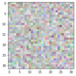
Glow
कागज से एक bijector उलटी 1x1 convolutions के साथ उत्पादक प्रवाह: चमक , किंगमा और धारीवाल द्वारा।
यहां वितरण से छवि बनाने का तरीका बताया गया है (ध्यान दें कि वितरण ने यहां कुछ भी "सीखा" नहीं है)।
image_shape = (32, 32, 4)  # 32 x 32 RGBA image

glow = tfb.Glow(output_shape=image_shape,
                coupling_bijector_fn=tfb.GlowDefaultNetwork,
                exit_bijector_fn=tfb.GlowDefaultExitNetwork)

pz = tfd.Sample(tfd.Normal(0., 1.), tf.reduce_prod(image_shape))

# Calling glow on distribution p(z) creates our glow distribution over images.
px = glow(pz)

# Take samples from the distribution to get images from your dataset.
image = px.sample(1)[0].numpy()

# Rescale to [0, 1].
image = (image - image.min()) / (image.max() - image.min())
plt.imshow(image);
RayleighCDF
के लिए Bijector रेले वितरण के CDF। एक उपयोग रेले वितरण से नमूना लेना है, एक समान नमूने लेकर, फिर उन्हें सीडीएफ के व्युत्क्रम से गुजरना।
bij = tfb.RayleighCDF()
uniforms = tfd.Uniform().sample(10_000)
plt.hist(bij.inverse(uniforms), bins='auto');

Ascending() की जगह Invert(Ordered())
x = tfd.Normal(0., 1.).sample(5)
print(tfb.Ascending()(x))
print(tfb.Invert(tfb.Ordered())(x))
tf.Tensor([1.9363368 2.650928  3.4936204 4.1817293 5.6920815], shape=(5,), dtype=float32)
WARNING:tensorflow:From <ipython-input-5-1406b9939c00>:3: Ordered.__init__ (from tensorflow_probability.python.bijectors.ordered) is deprecated and will be removed after 2021-01-09.
Instructions for updating:
`Ordered` bijector is deprecated; please use `tfb.Invert(tfb.Ascending())` instead.
tf.Tensor([1.9363368 2.650928  3.4936204 4.1817293 5.6920815], shape=(5,), dtype=float32)
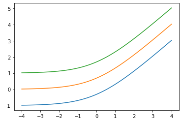
जोड़े low आर्ग: Softplus(low=2.)
x = tf.linspace(-4., 4., 100)

for low in (-1., 0., 1.):
  bij = tfb.Softplus(low=low)
  plt.plot(x, bij(x));
tfb.ScaleMatvecLinearOperatorBlock blockwise का समर्थन करता है LinearOperator , बहु-भाग आर्ग
op_1 = tf.linalg.LinearOperatorDiag(diag=[1., -1., 3.])
op_2 = tf.linalg.LinearOperatorFullMatrix([[12., 5.], [-1., 3.]])
scale = tf.linalg.LinearOperatorBlockDiag([op_1, op_2], is_non_singular=True)

bij = tfb.ScaleMatvecLinearOperatorBlock(scale)
bij([[1., 2., 3.], [0., 1.]])
WARNING:tensorflow:From /usr/local/lib/python3.6/dist-packages/tensorflow/python/ops/linalg/linear_operator_block_diag.py:223: LinearOperator.graph_parents (from tensorflow.python.ops.linalg.linear_operator) is deprecated and will be removed in a future version.
Instructions for updating:
Do not call `graph_parents`.
[<tf.Tensor: shape=(3,), dtype=float32, numpy=array([ 1., -2.,  9.], dtype=float32)>,
 <tf.Tensor: shape=(2,), dtype=float32, numpy=array([5., 3.], dtype=float32)>]
वितरण
Skellam
दो के अंतर से अधिक वितरण Poisson RVs। ध्यान दें कि इस वितरण से नमूने नकारात्मक हो सकते हैं।
x = tf.linspace(-5., 10., 10 - -5 + 1)

rates = (4, 2)
for i, rate in enumerate(rates):
  plt.bar(x - .3 * (1 - i), tfd.Poisson(rate).prob(x), label=f'Poisson({rate})', alpha=0.5, width=.3)
plt.bar(x.numpy() + .3, tfd.Skellam(*rates).prob(x).numpy(), color='k', alpha=0.25, width=.3,
        label=f'Skellam{rates}')

plt.legend();

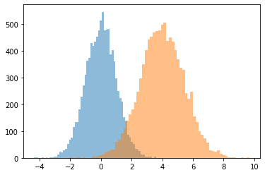
JointDistributionCoroutine[AutoBatched] उत्पादन namedtuple तरह के नमूने
स्पष्ट रूप से निर्दिष्ट sample_dtype=[...] वर्ष के लिए tuple व्यवहार।
@tfd.JointDistributionCoroutineAutoBatched
def model():
  x = yield tfd.Normal(0., 1., name='x')
  y = x + 4.
  yield tfd.Normal(y, 1., name='y')

draw = model.sample(10_000)

plt.hist(draw.x, bins='auto', alpha=0.5)
plt.hist(draw.y, bins='auto', alpha=0.5);
WARNING:tensorflow:Note that RandomStandardNormal inside pfor op may not give same output as inside a sequential loop.
WARNING:tensorflow:Note that RandomStandardNormal inside pfor op may not give same output as inside a sequential loop.
VonMisesFisher का समर्थन करता है dim > 5 , entropy()
वॉन Mises-फिशर वितरण पर एक वितरण है \(n-1\) में आयामी क्षेत्र \(\mathbb{R}^n\)।
dist = tfd.VonMisesFisher([0., 1, 0, 1, 0, 1], concentration=1.)
draws = dist.sample(3)

print(dist.entropy())
tf.reduce_sum(draws ** 2, axis=1)  # each draw has length 1
tf.Tensor(3.3533673, shape=(), dtype=float32)
<tf.Tensor: shape=(3,), dtype=float32, numpy=array([1.0000002 , 0.99999994, 1.0000001 ], dtype=float32)>
ExpGamma , ExpInverseGamma
log_rate पैरामीटर को जोड़ा गया Gamma । संख्यात्मक सुधार जब कम एकाग्रता नमूने Beta , Dirichlet और दोस्तों। सभी मामलों में लागू पुनरावर्तन ग्रेडिएंट।
plt.figure(figsize=(10, 3))
plt.subplot(121)
plt.hist(tfd.Beta(.02, .02).sample(10_000), bins='auto')
plt.title('Beta(.02, .02)')
plt.subplot(122)
plt.title('GamX/(GamX+GamY) [the old way]')
g = tfd.Gamma(.02, 1); s0, s1 = g.sample(10_000), g.sample(10_000)
plt.hist(s0 / (s0 + s1), bins='auto')
plt.show()

plt.figure(figsize=(10, 3))
plt.subplot(121)
plt.hist(tfd.ExpGamma(.02, 1.).sample(10_000), bins='auto')
plt.title('ExpGamma(.02, 1)')
plt.subplot(122)
plt.hist(tfb.Log()(tfd.Gamma(.02, 1.)).sample(10_000), bins='auto')
plt.title('tfb.Log()(Gamma(.02, 1)) [the old way]');


JointDistribution*AutoBatched समर्थन प्रतिलिपि प्रस्तुत करने योग्य नमूना (लंबाई -2 टपल साथ / टेन्सर बीज)
@tfd.JointDistributionCoroutineAutoBatched
def model():
  x = yield tfd.Normal(0, 1, name='x')
  y = yield tfd.Normal(x + 4, 1, name='y')

print(model.sample(seed=(1, 2)))
print(model.sample(seed=(1, 2)))
StructTuple(
  x=<tf.Tensor: shape=(), dtype=float32, numpy=-0.59835213>,
  y=<tf.Tensor: shape=(), dtype=float32, numpy=6.2380724>
)
StructTuple(
  x=<tf.Tensor: shape=(), dtype=float32, numpy=-0.59835213>,
  y=<tf.Tensor: shape=(), dtype=float32, numpy=6.2380724>
)
KL(VonMisesFisher || SphericalUniform)
# Build vMFs with the same mean direction, batch of increasing concentrations.
vmf = tfd.VonMisesFisher(tf.math.l2_normalize(tf.random.normal([10])),
                         concentration=[0., .1, 1., 10.])
# KL increases with concentration, since vMF(conc=0) == SphericalUniform.
print(tfd.kl_divergence(vmf, tfd.SphericalUniform(10)))
tf.Tensor([4.7683716e-07 4.9877167e-04 4.9384594e-02 2.4844694e+00], shape=(4,), dtype=float32)
parameter_properties
वितरण कक्षाएं अब एक बेनकाब parameter_properties(dtype=tf.float32, num_classes=None) वर्ग विधि है, जो वितरण के कई वर्गों में से स्वचालित निर्माण सक्षम कर सकते हैं।
print('Gamma:', tfd.Gamma.parameter_properties())
print('Categorical:', tfd.Categorical.parameter_properties(dtype=tf.float64, num_classes=7))
Gamma: {'concentration': ParameterProperties(event_ndims=0, shape_fn=<function ParameterProperties.<lambda> at 0x7ff6bbfcdd90>, default_constraining_bijector_fn=<function Gamma._parameter_properties.<locals>.<lambda> at 0x7ff6afd95510>, is_preferred=True), 'rate': ParameterProperties(event_ndims=0, shape_fn=<function ParameterProperties.<lambda> at 0x7ff6bbfcdd90>, default_constraining_bijector_fn=<function Gamma._parameter_properties.<locals>.<lambda> at 0x7ff6afd95ea0>, is_preferred=False), 'log_rate': ParameterProperties(event_ndims=0, shape_fn=<function ParameterProperties.<lambda> at 0x7ff6bbfcdd90>, default_constraining_bijector_fn=<class 'tensorflow_probability.python.bijectors.identity.Identity'>, is_preferred=True)}
Categorical: {'logits': ParameterProperties(event_ndims=1, shape_fn=<function Categorical._parameter_properties.<locals>.<lambda> at 0x7ff6afd95510>, default_constraining_bijector_fn=<class 'tensorflow_probability.python.bijectors.identity.Identity'>, is_preferred=True), 'probs': ParameterProperties(event_ndims=1, shape_fn=<function Categorical._parameter_properties.<locals>.<lambda> at 0x7ff6afdc91e0>, default_constraining_bijector_fn=<class 'tensorflow_probability.python.bijectors.softmax_centered.SoftmaxCentered'>, is_preferred=False)}
experimental_default_event_space_bijector
अब कुछ वितरण भागों को पिन करते हुए अतिरिक्त आर्ग स्वीकार करता है।
@tfd.JointDistributionCoroutineAutoBatched
def model():
  scale = yield tfd.Gamma(1, 1, name='scale')
  obs = yield tfd.Normal(0, scale, name='obs')

model.experimental_default_event_space_bijector(obs=.2).forward(
    [tf.random.uniform([3], -2, 2.)])
StructTuple(
  scale=<tf.Tensor: shape=(3,), dtype=float32, numpy=array([0.6630705, 1.5401832, 1.0777743], dtype=float32)>
)
JointDistribution.experimental_pin
पिंस कुछ संयुक्त वितरण भागों, लौटने JointDistributionPinned वस्तु संयुक्त unnormalized घनत्व का प्रतिनिधित्व।
के साथ कार्य करना experimental_default_event_space_bijector , इस समझदार चूक के साथ परिवर्तन संबंधी अनुमान या एमसीएमसी कर बनाता है और अधिक सरल। उदाहरण नीचे में, के पहले दो लाइनों sample बना एमसीएमसी चल रहा एक हवा।
dist = tfd.JointDistributionSequential([
    tfd.HalfNormal(1.),
    lambda scale: tfd.Normal(0., scale, name='observed')])

@tf.function
def sample():
  bij = dist.experimental_default_event_space_bijector(observed=1.)
  target_log_prob = dist.experimental_pin(observed=1.).unnormalized_log_prob

  kernel = tfp.mcmc.TransformedTransitionKernel(
      tfp.mcmc.HamiltonianMonteCarlo(target_log_prob,
                                     step_size=0.6,
                                     num_leapfrog_steps=16),
      bijector=bij)
  return tfp.mcmc.sample_chain(500,
                               current_state=tf.ones([8]),  # multiple chains
                               kernel=kernel,
                               trace_fn=None)

draws = sample()

fig, (hist, trace) = plt.subplots(ncols=2, figsize=(16, 3))
trace.plot(draws, alpha=0.5)
for col in tf.transpose(draws):
  sns.kdeplot(col, ax=hist);

tfd.NegativeBinomial.experimental_from_mean_dispersion
वैकल्पिक पैरामीटरकरण। ईमेल tfprobability@tensorflow.org या अन्य वितरणों के लिए समान वर्ग विधियों को जोड़ने के लिए हमें एक पीआर भेजें।
nb = tfd.NegativeBinomial.experimental_from_mean_dispersion(30., .01)
plt.hist(nb.sample(10_000), bins='auto');

tfp.experimental.distribute
DistributionStrategy संयुक्त वितरण -aware, क्रॉस-उपकरण संभावना संगणना के लिए अनुमति देता है। Sharded Independent और Sample वितरण।
# Note: 2-logical devices are configured in the install/import cell at top.
strategy = tf.distribute.MirroredStrategy()
assert strategy.num_replicas_in_sync == 2

@tfp.experimental.distribute.JointDistributionCoroutine
def model():
  root = tfp.experimental.distribute.JointDistributionCoroutine.Root
  group_scale = yield root(tfd.Sample(tfd.Exponential(1), 3, name='group_scale'))
  _ = yield tfp.experimental.distribute.ShardedSample(tfd.Independent(tfd.Normal(0, group_scale), 1),
                                                      sample_shape=[4], name='x')

seed1, seed2 = tfp.random.split_seed((1, 2))

@tf.function
def sample(seed):
  return model.sample(seed=seed)
xs = strategy.run(sample, (seed1,))
print("""
Note that the global latent `group_scale` is shared across devices, whereas
the local `x` is sampled independently on each device.
""")
print('sample:', xs)
print('another sample:', strategy.run(sample, (seed2,)))

@tf.function
def log_prob(x):
  return model.log_prob(x)
print("""
Note that each device observes the same log_prob (local latent log_probs are
summed across devices).
""")
print('log_prob:', strategy.run(log_prob, (xs,)))

@tf.function
def grad_log_prob(x):
  return tfp.math.value_and_gradient(model.log_prob, x)[1]

print("""
Note that each device observes the same log_prob gradient (local latents have
independent gradients, global latents have gradients aggregated across devices).
""")
print('grad_log_prob:', strategy.run(grad_log_prob, (xs,)))
WARNING:tensorflow:There are non-GPU devices in `tf.distribute.Strategy`, not using nccl allreduce.
INFO:tensorflow:Using MirroredStrategy with devices ('/job:localhost/replica:0/task:0/device:CPU:0', '/job:localhost/replica:0/task:0/device:CPU:1')

Note that the global latent `group_scale` is shared across devices, whereas
the local `x` is sampled independently on each device.

sample: StructTuple(
  group_scale=PerReplica:{
      0: <tf.Tensor: shape=(3,), dtype=float32, numpy=array([2.6355493, 1.1805456, 1.245112 ], dtype=float32)>,
      1: <tf.Tensor: shape=(3,), dtype=float32, numpy=array([2.6355493, 1.1805456, 1.245112 ], dtype=float32)>
    },
  x=PerReplica:{
      0: <tf.Tensor: shape=(2, 3), dtype=float32, numpy=
    array([[-0.90548456,  0.7675636 ,  0.27627748],
           [-0.3475989 ,  2.0194046 , -1.2531326 ]], dtype=float32)>,
      1: <tf.Tensor: shape=(2, 3), dtype=float32, numpy=
    array([[ 3.251305  , -0.5790973 ,  0.42745453],
           [-1.562331  ,  0.3006323 ,  0.635732  ]], dtype=float32)>
    }
)
another sample: StructTuple(
  group_scale=PerReplica:{
      0: <tf.Tensor: shape=(3,), dtype=float32, numpy=array([2.41133   , 0.10307606, 0.5236566 ], dtype=float32)>,
      1: <tf.Tensor: shape=(3,), dtype=float32, numpy=array([2.41133   , 0.10307606, 0.5236566 ], dtype=float32)>
    },
  x=PerReplica:{
      0: <tf.Tensor: shape=(2, 3), dtype=float32, numpy=
    array([[-3.2476294 ,  0.07213175, -0.39536062],
           [-1.2319602 , -0.05505352,  0.06356457]], dtype=float32)>,
      1: <tf.Tensor: shape=(2, 3), dtype=float32, numpy=
    array([[ 5.6028705 ,  0.11919801, -0.48446828],
           [-1.5938259 ,  0.21123725,  0.28979057]], dtype=float32)>
    }
)

Note that each device observes the same log_prob (local latent log_probs are
summed across devices).

INFO:tensorflow:Reduce to /job:localhost/replica:0/task:0/device:CPU:0 then broadcast to ('/job:localhost/replica:0/task:0/device:CPU:0', '/job:localhost/replica:0/task:0/device:CPU:1').
log_prob: PerReplica:{
  0: tf.Tensor(-25.05747, shape=(), dtype=float32),
  1: tf.Tensor(-25.05747, shape=(), dtype=float32)
}

Note that each device observes the same log_prob gradient (local latents have
independent gradients, global latents are aggregated across devices).

INFO:tensorflow:Reduce to /job:localhost/replica:0/task:0/device:CPU:0 then broadcast to ('/job:localhost/replica:0/task:0/device:CPU:0', '/job:localhost/replica:0/task:0/device:CPU:1').
INFO:tensorflow:Reduce to /job:localhost/replica:0/task:0/device:CPU:0 then broadcast to ('/job:localhost/replica:0/task:0/device:CPU:0', '/job:localhost/replica:0/task:0/device:CPU:1').
grad_log_prob: StructTuple(
  group_scale=PerReplica:{
      0: <tf.Tensor: shape=(3,), dtype=float32, numpy=array([-1.7555585, -1.2928739, -3.0554674], dtype=float32)>,
      1: <tf.Tensor: shape=(3,), dtype=float32, numpy=array([-1.7555585, -1.2928739, -3.0554674], dtype=float32)>
    },
  x=PerReplica:{
      0: <tf.Tensor: shape=(2, 3), dtype=float32, numpy=
    array([[ 0.13035832, -0.5507428 , -0.17820862],
           [ 0.05004217, -1.4489648 ,  0.80831426]], dtype=float32)>,
      1: <tf.Tensor: shape=(2, 3), dtype=float32, numpy=
    array([[-0.46807498,  0.41551432, -0.27572307],
           [ 0.22492138, -0.21570992, -0.41006932]], dtype=float32)>
    }
)
PSD गुठली
GeneralizedMatern
GeneralizedMatern सकारात्मक-semidefinite गिरी सामान्यीकरण करता MaternOneHalf , MAterhThreeHalves , और MaternFiveHalves ।
gm = tfpk.GeneralizedMatern(df=[0.5, 1.5, 2.5], length_scale=1., amplitude=0.5)
m1 = tfpk.MaternOneHalf(length_scale=1., amplitude=0.5)
m2 = tfpk.MaternThreeHalves(length_scale=1., amplitude=0.5)
m3 = tfpk.MaternFiveHalves(length_scale=1., amplitude=0.5)
xs = tf.linspace(-1.5, 1.5, 100)

gm_matrix = gm.matrix([[0.]], xs[..., tf.newaxis])
plt.plot(xs, gm_matrix[0][0])
plt.plot(xs, m1.matrix([[0.]], xs[..., tf.newaxis])[0])
plt.show()
plt.plot(xs, gm_matrix[1][0])
plt.plot(xs, m2.matrix([[0.]], xs[..., tf.newaxis])[0])
plt.show()
plt.plot(xs, gm_matrix[2][0])
plt.plot(xs, m3.matrix([[0.]], xs[..., tf.newaxis])[0])
plt.show()


Parabolic (Epanechnikov)
epa = tfpk.Parabolic()
xs = tf.linspace(-1.05, 1.05, 100)
plt.plot(xs, epa.matrix([[0.]], xs[..., tf.newaxis])[0]);

छठी
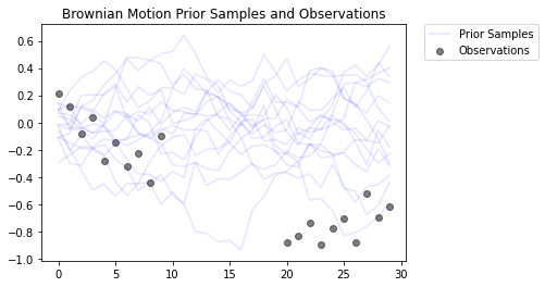
build_asvi_surrogate_posterior
VI के लिए स्वचालित रूप से एक संरचित सरोगेट पोस्टीरियर का निर्माण इस तरह से करें जिसमें पूर्व वितरण की चित्रमय संरचना शामिल हो। इस विधि कागज स्वत: संरचित परिवर्तन संबंधी निष्कर्ष (में वर्णित का इस्तेमाल करता https://arxiv.org/abs/2002.00643 )।
# Import a Brownian Motion model from TFP's inference gym.
model = gym.targets.BrownianMotionMissingMiddleObservations()
prior = model.prior_distribution()
ground_truth = ground_truth = model.sample_transformations['identity'].ground_truth_mean
target_log_prob = lambda *values: model.log_likelihood(values) + prior.log_prob(values)
यह गाऊसी प्रेक्षण मॉडल के साथ ब्राउनियन मोशन प्रक्रिया को मॉडल करता है। इसमें 30 टाइमस्टेप्स होते हैं, लेकिन बीच के 10 टाइमस्टेप्स देखने योग्य नहीं होते हैं।
  locs[0] ~ Normal(loc=0, scale=innovation_noise_scale)
  for t in range(1, num_timesteps):
    locs[t] ~ Normal(loc=locs[t - 1], scale=innovation_noise_scale)

  for t in range(num_timesteps):
    observed_locs[t] ~ Normal(loc=locs[t], scale=observation_noise_scale)
लक्ष्य के मूल्यों का अनुमान लगा रहा है locs शोर टिप्पणियों (से observed_locs )। के बाद से मध्य 10 timesteps सर्वनाश कर रहे हैं, observed_locs हैं NaN timesteps [10,19] में मान।
# The observed loc values in the Brownian Motion inference gym model
OBSERVED_LOC = np.array([
    0.21592641, 0.118771404, -0.07945447, 0.037677474, -0.27885845, -0.1484156,
    -0.3250906, -0.22957903, -0.44110894, -0.09830782, np.nan, np.nan, np.nan,
    np.nan, np.nan, np.nan, np.nan, np.nan, np.nan, np.nan, -0.8786016,
    -0.83736074, -0.7384849, -0.8939254, -0.7774566, -0.70238715, -0.87771565,
    -0.51853573, -0.6948214, -0.6202789
]).astype(dtype=np.float32)

# Plot the prior and the likelihood observations
plt.figure()
plt.title('Brownian Motion Prior Samples and Observations')

num_samples = 15
prior_samples = prior.sample(num_samples)

plt.plot(prior_samples, c='blue', alpha=0.1)
plt.plot(prior_samples[0][0], label="Prior Samples", c='blue', alpha=0.1)

plt.scatter(x=range(30),y=OBSERVED_LOC, c='black', alpha=0.5, label="Observations")

plt.legend(bbox_to_anchor=(1.05, 1), borderaxespad=0.);
logging.getLogger('tensorflow').setLevel(logging.ERROR)  # suppress pfor warnings

# Construct and train an ASVI Surrogate Posterior.
asvi_surrogate_posterior = tfp.experimental.vi.build_asvi_surrogate_posterior(prior)

asvi_losses = tfp.vi.fit_surrogate_posterior(target_log_prob,
                                        asvi_surrogate_posterior,
                                        optimizer=tf.optimizers.Adam(learning_rate=0.1),
                                        num_steps=500)
logging.getLogger('tensorflow').setLevel(logging.NOTSET)
# Construct and train a Mean-Field Surrogate Posterior.
factored_surrogate_posterior = tfp.experimental.vi.build_factored_surrogate_posterior(event_shape=prior.event_shape)

factored_losses = tfp.vi.fit_surrogate_posterior(target_log_prob,
                                        factored_surrogate_posterior,
                                        optimizer=tf.optimizers.Adam(learning_rate=0.1),
                                        num_steps=500)
logging.getLogger('tensorflow').setLevel(logging.ERROR)  # suppress pfor warnings

# Sample from the posteriors.
asvi_posterior_samples = asvi_surrogate_posterior.sample(num_samples)
factored_posterior_samples = factored_surrogate_posterior.sample(num_samples)

logging.getLogger('tensorflow').setLevel(logging.NOTSET)
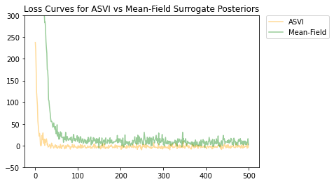
ASVI और माध्य-क्षेत्र सरोगेट पश्च वितरण दोनों अभिसरण हो गए हैं, और ASVI सरोगेट पोस्टीरियर में कम अंतिम नुकसान (नकारात्मक ELBO मान) था।
# Plot the loss curves.
plt.figure()
plt.title('Loss Curves for ASVI vs Mean-Field Surrogate Posteriors')

plt.plot(asvi_losses, c='orange', label='ASVI', alpha = 0.4)
plt.plot(factored_losses, c='green', label='Mean-Field', alpha = 0.4)
plt.ylim(-50, 300)

plt.legend(bbox_to_anchor=(1.3, 1), borderaxespad=0.);
पोस्टरियर के नमूने इस बात पर प्रकाश डालते हैं कि ASVI सरोगेट पोस्टीरियर कितनी अच्छी तरह से टिप्पणियों के बिना टाइमस्टेप्स के लिए अनिश्चितता को पकड़ लेता है। दूसरी ओर, वास्तविक अनिश्चितता को पकड़ने के लिए माध्य-क्षेत्र सरोगेट पश्च-संघर्ष करता है।
# Plot samples from the ASVI and Mean-Field Surrogate Posteriors.
plt.figure()
plt.title('Posterior Samples from ASVI vs Mean-Field Surrogate Posterior')

plt.plot(asvi_posterior_samples, c='orange', alpha = 0.25)
plt.plot(asvi_posterior_samples[0][0], label='ASVI Surrogate Posterior', c='orange', alpha = 0.25)

plt.plot(factored_posterior_samples, c='green', alpha = 0.25)
plt.plot(factored_posterior_samples[0][0], label='Mean-Field Surrogate Posterior', c='green', alpha = 0.25)

plt.scatter(x=range(30),y=OBSERVED_LOC, c='black', alpha=0.5, label='Observations')

plt.plot(ground_truth, c='black', label='Ground Truth')

plt.legend(bbox_to_anchor=(1.585, 1), borderaxespad=0.);

एमसीएमसी
ProgressBarReducer
सैम्पलर की प्रगति की कल्पना करें। (एक मामूली प्रदर्शन जुर्माना हो सकता है; वर्तमान में जेआईटी संकलन के तहत समर्थित नहीं है।)
kernel = tfp.mcmc.HamiltonianMonteCarlo(lambda x: -x**2 / 2, .05, 20)
pbar = tfp.experimental.mcmc.ProgressBarReducer(100)
kernel = tfp.experimental.mcmc.WithReductions(kernel, pbar)
plt.hist(tf.reshape(tfp.mcmc.sample_chain(100, current_state=tf.ones([128]), kernel=kernel, trace_fn=None), [-1]), bins='auto')
pbar.bar.close()
99%|█████████▉| 99/100 [00:03<00:00, 27.37it/s]
sample_sequential_monte_carlo प्रतिलिपि प्रस्तुत करने योग्य नमूना का समर्थन करता है
initial_state = tf.random.uniform([4096], -2., 2.)
def smc(seed):
  return tfp.experimental.mcmc.sample_sequential_monte_carlo(
    prior_log_prob_fn=lambda x: -x**2 / 2,
    likelihood_log_prob_fn=lambda x: -(x-1.)**2 / 2,
    current_state=initial_state,
    seed=seed)[1]
plt.hist(smc(seed=(12, 34)), bins='auto');plt.show()

print(smc(seed=(12, 34))[:10])
print('different:', smc(seed=(10, 20))[:10])
print('same:', smc(seed=(12, 34))[:10])

tf.Tensor(
[ 0.665834    0.9892149   0.7961128   1.0016634  -1.000767   -0.19461267
  1.3070581   1.127177    0.9940303   0.58239716], shape=(10,), dtype=float32)
different: tf.Tensor(
[ 1.3284367   0.4374407   1.1349089   0.4557473   0.06510283 -0.08954388
  1.1735026   0.8170528   0.12443061  0.34413314], shape=(10,), dtype=float32)
same: tf.Tensor(
[ 0.665834    0.9892149   0.7961128   1.0016634  -1.000767   -0.19461267
  1.3070581   1.127177    0.9940303   0.58239716], shape=(10,), dtype=float32)
विचरण, सहप्रसरण, रहट की स्ट्रीमिंग संगणना जोड़ी गई
ध्यान दें, इन करने के लिए इंटरफेस में कुछ हद तक बदल दिया है tfp-nightly ।
def cov_to_ellipse(t, cov, mean):
  """Draw a one standard deviation ellipse from the mean, according to cov."""
  diag = tf.linalg.diag_part(cov)
  a = 0.5 * tf.reduce_sum(diag)
  b = tf.sqrt(0.25 * (diag[0] - diag[1])**2 + cov[0, 1]**2)
  major = a + b
  minor = a - b
  theta = tf.math.atan2(major - cov[0, 0], cov[0, 1])
  x = (tf.sqrt(major) * tf.cos(theta) * tf.cos(t) -
       tf.sqrt(minor) * tf.sin(theta) * tf.sin(t))
  y = (tf.sqrt(major) * tf.sin(theta) * tf.cos(t) +
       tf.sqrt(minor) * tf.cos(theta) * tf.sin(t))
  return x + mean[0], y + mean[1]

fig, axes = plt.subplots(nrows=4, ncols=5, figsize=(14, 8),
                         sharex=True, sharey=True, constrained_layout=True)
t = tf.linspace(0., 2 * np.pi, 200)
tot = 10
cov = 0.1 * tf.eye(2) + 0.9 * tf.ones([2, 2])
mvn = tfd.MultivariateNormalTriL(loc=[1., 2.],
                                 scale_tril=tf.linalg.cholesky(cov))

for ax in axes.ravel():
  rv = tfp.experimental.stats.RunningCovariance(
      num_samples=0., mean=tf.zeros(2), sum_squared_residuals=tf.zeros((2, 2)),
      event_ndims=1)

  for idx, x in enumerate(mvn.sample(tot)):
    rv = rv.update(x)
    ax.plot(*cov_to_ellipse(t, rv.covariance(), rv.mean),
            color='k', alpha=(idx + 1) / tot)
  ax.plot(*cov_to_ellipse(t, mvn.covariance(), mvn.mean()), 'r')
fig.suptitle("Twenty tries to approximate the red covariance with 10 draws");

गणित, आँकड़े
बेसेल फ़ंक्शन: ive, kve, log-ive
xs = tf.linspace(0.5, 20., 100)
ys = tfp.math.bessel_ive([[0.5], [1.], [np.pi], [4.]], xs)
zs = tfp.math.bessel_kve([[0.5], [1.], [2.], [np.pi]], xs)

for i in range(4):
  plt.plot(xs, ys[i])
plt.show()

for i in range(4):
  plt.plot(xs, zs[i])
plt.show()


वैकल्पिक weights को ARG tfp.stats.histogram
edges = tf.linspace(-4., 4, 31)
samps = tfd.TruncatedNormal(0, 1, -4, 4).sample(100_000, seed=(123, 456))
_, (ax1, ax2) = plt.subplots(1, 2, figsize=(10, 3))
ax1.bar(edges[:-1], tfp.stats.histogram(samps, edges))
ax1.set_title('samples histogram')
ax2.bar(edges[:-1], tfp.stats.histogram(samps, edges, weights=1 / tfd.Normal(0, 1).prob(samps)))
ax2.set_title('samples, weighted by inverse p(sample)');

tfp.math.erfcinv
x = tf.linspace(-3., 3., 10)
y = tf.math.erfc(x)
z = tfp.math.erfcinv(y)
print(x)
print(z)
tf.Tensor(
[-3.         -2.3333333  -1.6666666  -1.         -0.33333325  0.3333335

  1.          1.666667    2.3333335   3.        ], shape=(10,), dtype=float32)
tf.Tensor(
[-3.0002644  -2.3333426  -1.6666666  -0.9999997  -0.3333332   0.33333346
  0.9999999   1.6666667   2.3333335   3.0000002 ], shape=(10,), dtype=float32)