
| | |  Xem trên GitHub Xem trên GitHub | |
Trong các ứng dụng AI quan trọng đến an toàn (ví dụ: ra quyết định y tế và lái xe tự động) hoặc nơi dữ liệu vốn đã bị nhiễu (ví dụ: hiểu ngôn ngữ tự nhiên), điều quan trọng là một bộ phân loại sâu phải định lượng một cách đáng tin cậy độ không chắc chắn của nó. Bộ phân loại sâu phải có khả năng nhận thức được những hạn chế của chính nó và khi nào nó nên giao quyền kiểm soát cho các chuyên gia con người. Hướng dẫn này chỉ ra cách cải thiện khả năng của bộ phân loại sâu trong việc định lượng độ không đảm bảo bằng cách sử dụng kỹ thuật gọi là Quy trình Gaussian thần kinh chuẩn hóa phổ ( SNGP ) .
Ý tưởng cốt lõi của SNGP là cải thiện nhận thức về khoảng cách của bộ phân loại sâu bằng cách áp dụng các sửa đổi đơn giản cho mạng. Nhận thức về khoảng cách của một mô hình là thước đo xác suất dự đoán của nó phản ánh khoảng cách giữa ví dụ thử nghiệm và dữ liệu đào tạo như thế nào. Đây là đặc tính mong muốn phổ biến đối với các mô hình xác suất tiêu chuẩn vàng (ví dụ: quy trình Gaussian với hạt nhân RBF) nhưng lại thiếu trong các mô hình có mạng nơron sâu. SNGP cung cấp một cách đơn giản để đưa hành vi của quy trình Gaussian này vào một bộ phân loại sâu trong khi vẫn duy trì độ chính xác dự đoán của nó.
Hướng dẫn này triển khai mô hình SNGP dựa trên mạng phần dư sâu (ResNet) trên tập dữ liệu hai mặt trăng và so sánh bề mặt không chắc chắn của nó với hai phương pháp tiếp cận độ không đảm bảo phổ biến khác - Monte Carlo bỏ học và Tập hợp sâu ).
Hướng dẫn này minh họa mô hình SNGP trên tập dữ liệu 2D đồ chơi. Để biết ví dụ về việc áp dụng SNGP cho nhiệm vụ hiểu ngôn ngữ tự nhiên trong thế giới thực bằng cách sử dụng BERT-base, vui lòng xem hướng dẫn SNGP-BERT . Để triển khai chất lượng cao mô hình SNGP (và nhiều phương pháp độ không đảm bảo khác) trên nhiều bộ dữ liệu điểm chuẩn (ví dụ: CIFAR-100 , ImageNet , phát hiện độc tính Jigsaw , v.v.), vui lòng kiểm tra điểm chuẩn Đường cơ sở độ không đảm bảo.
Về SNGP
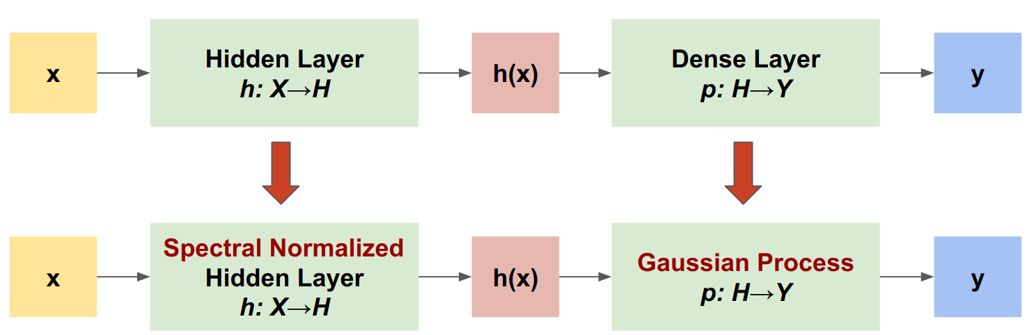
Quy trình Gaussian Neural được chuẩn hóa phổ (SNGP) là một cách tiếp cận đơn giản để cải thiện chất lượng độ không đảm bảo của bộ phân loại sâu trong khi vẫn duy trì mức độ chính xác và độ trễ tương tự. Với một mạng lưới dư sâu, SNGP thực hiện hai thay đổi đơn giản đối với mô hình:
- Nó áp dụng chuẩn hóa quang phổ cho các lớp dư ẩn.
- Nó thay thế lớp đầu ra dày đặc bằng lớp quy trình Gaussian.
So với các phương pháp tiếp cận không chắc chắn khác (ví dụ: Monte Carlo bỏ học hoặc Nhóm sâu), SNGP có một số lợi thế:
- Nó hoạt động cho một loạt các kiến trúc dựa trên phần dư hiện đại (ví dụ: (Wide) ResNet, DenseNet, BERT, v.v.).
- Đây là một phương pháp mô hình đơn (nghĩa là không dựa vào tính trung bình cộng). Do đó, SNGP có mức độ trễ tương tự như một mạng xác định duy nhất và có thể được mở rộng dễ dàng cho các tập dữ liệu lớn như ImageNet và phân loại Jigsaw Toxic Comments .
- Nó có hiệu suất phát hiện bên ngoài miền mạnh mẽ do thuộc tính nhận biết khoảng cách .
Nhược điểm của phương pháp này là:
Độ không đảm bảo dự đoán của SNGP được tính bằng phép gần đúng Laplace . Do đó về mặt lý thuyết, độ không đảm bảo đo hậu của SNGP khác với độ không đảm bảo đo của quá trình Gaussian chính xác.
Đào tạo SNGP cần một bước đặt lại hiệp phương sai khi bắt đầu một kỷ nguyên mới. Điều này có thể thêm một lượng nhỏ phức tạp thêm vào một đường dẫn đào tạo. Hướng dẫn này chỉ ra một cách đơn giản để thực hiện điều này bằng cách sử dụng các lệnh gọi lại của Keras.
Thành lập
pip install --use-deprecated=legacy-resolver tf-models-official
# refresh pkg_resources so it takes the changes into account.
import pkg_resources
import importlib
importlib.reload(pkg_resources)
<module 'pkg_resources' from '/tmpfs/src/tf_docs_env/lib/python3.7/site-packages/pkg_resources/__init__.py'>
import matplotlib.pyplot as plt
import matplotlib.colors as colors

import sklearn.datasets

import numpy as np
import tensorflow as tf

import official.nlp.modeling.layers as nlp_layers
Xác định macro trực quan hóa
plt.rcParams['figure.dpi'] = 140

DEFAULT_X_RANGE = (-3.5, 3.5)
DEFAULT_Y_RANGE = (-2.5, 2.5)
DEFAULT_CMAP = colors.ListedColormap(["#377eb8", "#ff7f00"])
DEFAULT_NORM = colors.Normalize(vmin=0, vmax=1,)
DEFAULT_N_GRID = 100
Bộ dữ liệu hai mặt trăng
Tạo tập dữ liệu đánh giá và trainining từ tập dữ liệu hai mặt trăng .
def make_training_data(sample_size=500):
  """Create two moon training dataset."""
  train_examples, train_labels = sklearn.datasets.make_moons(
      n_samples=2 * sample_size, noise=0.1)

  # Adjust data position slightly.
  train_examples[train_labels == 0] += [-0.1, 0.2]
  train_examples[train_labels == 1] += [0.1, -0.2]

  return train_examples, train_labels
Đánh giá hành vi dự đoán của mô hình trên toàn bộ không gian đầu vào 2D.
def make_testing_data(x_range=DEFAULT_X_RANGE, y_range=DEFAULT_Y_RANGE, n_grid=DEFAULT_N_GRID):
  """Create a mesh grid in 2D space."""
  # testing data (mesh grid over data space)
  x = np.linspace(x_range[0], x_range[1], n_grid)
  y = np.linspace(y_range[0], y_range[1], n_grid)
  xv, yv = np.meshgrid(x, y)
  return np.stack([xv.flatten(), yv.flatten()], axis=-1)
Để đánh giá độ không chắc chắn của mô hình, hãy thêm tập dữ liệu ngoài miền (OOD) thuộc về lớp thứ ba. Mô hình không bao giờ nhìn thấy các ví dụ OOD này trong quá trình đào tạo.
def make_ood_data(sample_size=500, means=(2.5, -1.75), vars=(0.01, 0.01)):
  return np.random.multivariate_normal(
      means, cov=np.diag(vars), size=sample_size)
# Load the train, test and OOD datasets.
train_examples, train_labels = make_training_data(
    sample_size=500)
test_examples = make_testing_data()
ood_examples = make_ood_data(sample_size=500)

# Visualize
pos_examples = train_examples[train_labels == 0]
neg_examples = train_examples[train_labels == 1]

plt.figure(figsize=(7, 5.5))

plt.scatter(pos_examples[:, 0], pos_examples[:, 1], c="#377eb8", alpha=0.5)
plt.scatter(neg_examples[:, 0], neg_examples[:, 1], c="#ff7f00", alpha=0.5)
plt.scatter(ood_examples[:, 0], ood_examples[:, 1], c="red", alpha=0.1)

plt.legend(["Postive", "Negative", "Out-of-Domain"])

plt.ylim(DEFAULT_Y_RANGE)
plt.xlim(DEFAULT_X_RANGE)

plt.show()

Ở đây, màu xanh lam và màu cam đại diện cho các lớp tích cực và tiêu cực, và màu đỏ đại diện cho dữ liệu OOD. Một mô hình định lượng tốt độ không đảm bảo sẽ tự tin khi gần với dữ liệu huấn luyện (tức là, \(p(x_{test})\) gần bằng 0 hoặc 1) và không chắc chắn khi ở xa vùng dữ liệu huấn luyện (tức là, \(p(x_{test})\) gần với 0.5 ).
Mô hình xác định
Xác định mô hình
Bắt đầu từ mô hình xác định (đường cơ sở): một mạng phần dư nhiều lớp (ResNet) với sự chính quy bỏ học.
class DeepResNet(tf.keras.Model):
  """Defines a multi-layer residual network."""
  def __init__(self, num_classes, num_layers=3, num_hidden=128,
               dropout_rate=0.1, **classifier_kwargs):
    super().__init__()
    # Defines class meta data.
    self.num_hidden = num_hidden
    self.num_layers = num_layers
    self.dropout_rate = dropout_rate
    self.classifier_kwargs = classifier_kwargs

    # Defines the hidden layers.
    self.input_layer = tf.keras.layers.Dense(self.num_hidden, trainable=False)
    self.dense_layers = [self.make_dense_layer() for _ in range(num_layers)]

    # Defines the output layer.
    self.classifier = self.make_output_layer(num_classes)

  def call(self, inputs):
    # Projects the 2d input data to high dimension.
    hidden = self.input_layer(inputs)

    # Computes the resnet hidden representations.
    for i in range(self.num_layers):
      resid = self.dense_layers[i](hidden)
      resid = tf.keras.layers.Dropout(self.dropout_rate)(resid)
      hidden += resid

    return self.classifier(hidden)

  def make_dense_layer(self):
    """Uses the Dense layer as the hidden layer."""
    return tf.keras.layers.Dense(self.num_hidden, activation="relu")

  def make_output_layer(self, num_classes):
    """Uses the Dense layer as the output layer."""
    return tf.keras.layers.Dense(
        num_classes, **self.classifier_kwargs)
Hướng dẫn này sử dụng ResNet 6 lớp với 128 đơn vị ẩn.
resnet_config = dict(num_classes=2, num_layers=6, num_hidden=128)
resnet_model = DeepResNet(**resnet_config)
resnet_model.build((None, 2))
resnet_model.summary()
Model: "deep_res_net"
_________________________________________________________________
 Layer (type)                Output Shape              Param #
=================================================================
 dense (Dense)               multiple                  384

 dense_1 (Dense)             multiple                  16512

 dense_2 (Dense)             multiple                  16512

 dense_3 (Dense)             multiple                  16512

 dense_4 (Dense)             multiple                  16512

 dense_5 (Dense)             multiple                  16512

 dense_6 (Dense)             multiple                  16512

 dense_7 (Dense)             multiple                  258

=================================================================
Total params: 99,714
Trainable params: 99,330
Non-trainable params: 384
_________________________________________________________________
Mô hình xe lửa
Định cấu hình các thông số huấn luyện để sử dụng SparseCategoricalCrossentropy làm hàm mất mát và trình tối ưu hóa Adam.
loss = tf.keras.losses.SparseCategoricalCrossentropy(from_logits=True)
metrics = tf.keras.metrics.SparseCategoricalAccuracy(),
optimizer = tf.keras.optimizers.Adam(learning_rate=1e-4)

train_config = dict(loss=loss, metrics=metrics, optimizer=optimizer)
Huấn luyện mô hình cho 100 kỷ nguyên với kích thước lô 128.
fit_config = dict(batch_size=128, epochs=100)
resnet_model.compile(**train_config)
resnet_model.fit(train_examples, train_labels, **fit_config)
Epoch 1/100
8/8 [==============================] - 1s 4ms/step - loss: 1.1251 - sparse_categorical_accuracy: 0.5050
Epoch 2/100
8/8 [==============================] - 0s 3ms/step - loss: 0.5538 - sparse_categorical_accuracy: 0.6920
Epoch 3/100
8/8 [==============================] - 0s 3ms/step - loss: 0.2881 - sparse_categorical_accuracy: 0.9160
Epoch 4/100
8/8 [==============================] - 0s 3ms/step - loss: 0.1923 - sparse_categorical_accuracy: 0.9370
Epoch 5/100
8/8 [==============================] - 0s 3ms/step - loss: 0.1550 - sparse_categorical_accuracy: 0.9420
Epoch 6/100
8/8 [==============================] - 0s 3ms/step - loss: 0.1403 - sparse_categorical_accuracy: 0.9450
Epoch 7/100
8/8 [==============================] - 0s 3ms/step - loss: 0.1269 - sparse_categorical_accuracy: 0.9430
Epoch 8/100
8/8 [==============================] - 0s 3ms/step - loss: 0.1208 - sparse_categorical_accuracy: 0.9460
Epoch 9/100
8/8 [==============================] - 0s 3ms/step - loss: 0.1158 - sparse_categorical_accuracy: 0.9510
Epoch 10/100
8/8 [==============================] - 0s 3ms/step - loss: 0.1103 - sparse_categorical_accuracy: 0.9490
Epoch 11/100
8/8 [==============================] - 0s 3ms/step - loss: 0.1051 - sparse_categorical_accuracy: 0.9510
Epoch 12/100
8/8 [==============================] - 0s 3ms/step - loss: 0.1053 - sparse_categorical_accuracy: 0.9510
Epoch 13/100
8/8 [==============================] - 0s 3ms/step - loss: 0.1013 - sparse_categorical_accuracy: 0.9450
Epoch 14/100
8/8 [==============================] - 0s 4ms/step - loss: 0.0967 - sparse_categorical_accuracy: 0.9500
Epoch 15/100
8/8 [==============================] - 0s 3ms/step - loss: 0.0991 - sparse_categorical_accuracy: 0.9530
Epoch 16/100
8/8 [==============================] - 0s 3ms/step - loss: 0.0984 - sparse_categorical_accuracy: 0.9500
Epoch 17/100
8/8 [==============================] - 0s 3ms/step - loss: 0.0982 - sparse_categorical_accuracy: 0.9480
Epoch 18/100
8/8 [==============================] - 0s 4ms/step - loss: 0.0918 - sparse_categorical_accuracy: 0.9510
Epoch 19/100
8/8 [==============================] - 0s 3ms/step - loss: 0.0903 - sparse_categorical_accuracy: 0.9500
Epoch 20/100
8/8 [==============================] - 0s 3ms/step - loss: 0.0883 - sparse_categorical_accuracy: 0.9510
Epoch 21/100
8/8 [==============================] - 0s 3ms/step - loss: 0.0870 - sparse_categorical_accuracy: 0.9530
Epoch 22/100
8/8 [==============================] - 0s 3ms/step - loss: 0.0884 - sparse_categorical_accuracy: 0.9560
Epoch 23/100
8/8 [==============================] - 0s 3ms/step - loss: 0.0850 - sparse_categorical_accuracy: 0.9540
Epoch 24/100
8/8 [==============================] - 0s 3ms/step - loss: 0.0808 - sparse_categorical_accuracy: 0.9580
Epoch 25/100
8/8 [==============================] - 0s 3ms/step - loss: 0.0773 - sparse_categorical_accuracy: 0.9560
Epoch 26/100
8/8 [==============================] - 0s 3ms/step - loss: 0.0801 - sparse_categorical_accuracy: 0.9590
Epoch 27/100
8/8 [==============================] - 0s 3ms/step - loss: 0.0779 - sparse_categorical_accuracy: 0.9580
Epoch 28/100
8/8 [==============================] - 0s 3ms/step - loss: 0.0807 - sparse_categorical_accuracy: 0.9580
Epoch 29/100
8/8 [==============================] - 0s 3ms/step - loss: 0.0820 - sparse_categorical_accuracy: 0.9570
Epoch 30/100
8/8 [==============================] - 0s 3ms/step - loss: 0.0730 - sparse_categorical_accuracy: 0.9600
Epoch 31/100
8/8 [==============================] - 0s 3ms/step - loss: 0.0782 - sparse_categorical_accuracy: 0.9590
Epoch 32/100
8/8 [==============================] - 0s 4ms/step - loss: 0.0704 - sparse_categorical_accuracy: 0.9600
Epoch 33/100
8/8 [==============================] - 0s 3ms/step - loss: 0.0709 - sparse_categorical_accuracy: 0.9610
Epoch 34/100
8/8 [==============================] - 0s 3ms/step - loss: 0.0758 - sparse_categorical_accuracy: 0.9580
Epoch 35/100
8/8 [==============================] - 0s 3ms/step - loss: 0.0702 - sparse_categorical_accuracy: 0.9610
Epoch 36/100
8/8 [==============================] - 0s 3ms/step - loss: 0.0688 - sparse_categorical_accuracy: 0.9600
Epoch 37/100
8/8 [==============================] - 0s 3ms/step - loss: 0.0675 - sparse_categorical_accuracy: 0.9630
Epoch 38/100
8/8 [==============================] - 0s 3ms/step - loss: 0.0636 - sparse_categorical_accuracy: 0.9690
Epoch 39/100
8/8 [==============================] - 0s 3ms/step - loss: 0.0677 - sparse_categorical_accuracy: 0.9610
Epoch 40/100
8/8 [==============================] - 0s 3ms/step - loss: 0.0702 - sparse_categorical_accuracy: 0.9650
Epoch 41/100
8/8 [==============================] - 0s 3ms/step - loss: 0.0614 - sparse_categorical_accuracy: 0.9690
Epoch 42/100
8/8 [==============================] - 0s 3ms/step - loss: 0.0663 - sparse_categorical_accuracy: 0.9680
Epoch 43/100
8/8 [==============================] - 0s 3ms/step - loss: 0.0626 - sparse_categorical_accuracy: 0.9740
Epoch 44/100
8/8 [==============================] - 0s 3ms/step - loss: 0.0590 - sparse_categorical_accuracy: 0.9760
Epoch 45/100
8/8 [==============================] - 0s 3ms/step - loss: 0.0573 - sparse_categorical_accuracy: 0.9780
Epoch 46/100
8/8 [==============================] - 0s 3ms/step - loss: 0.0568 - sparse_categorical_accuracy: 0.9770
Epoch 47/100
8/8 [==============================] - 0s 3ms/step - loss: 0.0595 - sparse_categorical_accuracy: 0.9780
Epoch 48/100
8/8 [==============================] - 0s 3ms/step - loss: 0.0482 - sparse_categorical_accuracy: 0.9840
Epoch 49/100
8/8 [==============================] - 0s 3ms/step - loss: 0.0515 - sparse_categorical_accuracy: 0.9820
Epoch 50/100
8/8 [==============================] - 0s 3ms/step - loss: 0.0525 - sparse_categorical_accuracy: 0.9830
Epoch 51/100
8/8 [==============================] - 0s 3ms/step - loss: 0.0507 - sparse_categorical_accuracy: 0.9790
Epoch 52/100
8/8 [==============================] - 0s 3ms/step - loss: 0.0433 - sparse_categorical_accuracy: 0.9850
Epoch 53/100
8/8 [==============================] - 0s 3ms/step - loss: 0.0511 - sparse_categorical_accuracy: 0.9820
Epoch 54/100
8/8 [==============================] - 0s 3ms/step - loss: 0.0501 - sparse_categorical_accuracy: 0.9820
Epoch 55/100
8/8 [==============================] - 0s 3ms/step - loss: 0.0440 - sparse_categorical_accuracy: 0.9890
Epoch 56/100
8/8 [==============================] - 0s 3ms/step - loss: 0.0438 - sparse_categorical_accuracy: 0.9850
Epoch 57/100
8/8 [==============================] - 0s 3ms/step - loss: 0.0438 - sparse_categorical_accuracy: 0.9880
Epoch 58/100
8/8 [==============================] - 0s 3ms/step - loss: 0.0416 - sparse_categorical_accuracy: 0.9860
Epoch 59/100
8/8 [==============================] - 0s 3ms/step - loss: 0.0479 - sparse_categorical_accuracy: 0.9860
Epoch 60/100
8/8 [==============================] - 0s 3ms/step - loss: 0.0434 - sparse_categorical_accuracy: 0.9860
Epoch 61/100
8/8 [==============================] - 0s 3ms/step - loss: 0.0414 - sparse_categorical_accuracy: 0.9880
Epoch 62/100
8/8 [==============================] - 0s 3ms/step - loss: 0.0402 - sparse_categorical_accuracy: 0.9870
Epoch 63/100
8/8 [==============================] - 0s 3ms/step - loss: 0.0376 - sparse_categorical_accuracy: 0.9890
Epoch 64/100
8/8 [==============================] - 0s 3ms/step - loss: 0.0337 - sparse_categorical_accuracy: 0.9900
Epoch 65/100
8/8 [==============================] - 0s 3ms/step - loss: 0.0309 - sparse_categorical_accuracy: 0.9910
Epoch 66/100
8/8 [==============================] - 0s 3ms/step - loss: 0.0336 - sparse_categorical_accuracy: 0.9910
Epoch 67/100
8/8 [==============================] - 0s 3ms/step - loss: 0.0389 - sparse_categorical_accuracy: 0.9870
Epoch 68/100
8/8 [==============================] - 0s 3ms/step - loss: 0.0333 - sparse_categorical_accuracy: 0.9920
Epoch 69/100
8/8 [==============================] - 0s 3ms/step - loss: 0.0331 - sparse_categorical_accuracy: 0.9890
Epoch 70/100
8/8 [==============================] - 0s 3ms/step - loss: 0.0346 - sparse_categorical_accuracy: 0.9900
Epoch 71/100
8/8 [==============================] - 0s 3ms/step - loss: 0.0367 - sparse_categorical_accuracy: 0.9880
Epoch 72/100
8/8 [==============================] - 0s 3ms/step - loss: 0.0283 - sparse_categorical_accuracy: 0.9920
Epoch 73/100
8/8 [==============================] - 0s 3ms/step - loss: 0.0315 - sparse_categorical_accuracy: 0.9930
Epoch 74/100
8/8 [==============================] - 0s 3ms/step - loss: 0.0271 - sparse_categorical_accuracy: 0.9900
Epoch 75/100
8/8 [==============================] - 0s 3ms/step - loss: 0.0257 - sparse_categorical_accuracy: 0.9920
Epoch 76/100
8/8 [==============================] - 0s 3ms/step - loss: 0.0289 - sparse_categorical_accuracy: 0.9900
Epoch 77/100
8/8 [==============================] - 0s 3ms/step - loss: 0.0264 - sparse_categorical_accuracy: 0.9900
Epoch 78/100
8/8 [==============================] - 0s 3ms/step - loss: 0.0272 - sparse_categorical_accuracy: 0.9910
Epoch 79/100
8/8 [==============================] - 0s 3ms/step - loss: 0.0336 - sparse_categorical_accuracy: 0.9880
Epoch 80/100
8/8 [==============================] - 0s 3ms/step - loss: 0.0249 - sparse_categorical_accuracy: 0.9900
Epoch 81/100
8/8 [==============================] - 0s 3ms/step - loss: 0.0216 - sparse_categorical_accuracy: 0.9930
Epoch 82/100
8/8 [==============================] - 0s 3ms/step - loss: 0.0279 - sparse_categorical_accuracy: 0.9890
Epoch 83/100
8/8 [==============================] - 0s 3ms/step - loss: 0.0261 - sparse_categorical_accuracy: 0.9920
Epoch 84/100
8/8 [==============================] - 0s 3ms/step - loss: 0.0235 - sparse_categorical_accuracy: 0.9920
Epoch 85/100
8/8 [==============================] - 0s 3ms/step - loss: 0.0236 - sparse_categorical_accuracy: 0.9930
Epoch 86/100
8/8 [==============================] - 0s 3ms/step - loss: 0.0219 - sparse_categorical_accuracy: 0.9920
Epoch 87/100
8/8 [==============================] - 0s 3ms/step - loss: 0.0196 - sparse_categorical_accuracy: 0.9920
Epoch 88/100
8/8 [==============================] - 0s 3ms/step - loss: 0.0215 - sparse_categorical_accuracy: 0.9900
Epoch 89/100
8/8 [==============================] - 0s 3ms/step - loss: 0.0223 - sparse_categorical_accuracy: 0.9900
Epoch 90/100
8/8 [==============================] - 0s 3ms/step - loss: 0.0200 - sparse_categorical_accuracy: 0.9950
Epoch 91/100
8/8 [==============================] - 0s 3ms/step - loss: 0.0250 - sparse_categorical_accuracy: 0.9900
Epoch 92/100
8/8 [==============================] - 0s 3ms/step - loss: 0.0160 - sparse_categorical_accuracy: 0.9940
Epoch 93/100
8/8 [==============================] - 0s 3ms/step - loss: 0.0203 - sparse_categorical_accuracy: 0.9930
Epoch 94/100
8/8 [==============================] - 0s 3ms/step - loss: 0.0203 - sparse_categorical_accuracy: 0.9930
Epoch 95/100
8/8 [==============================] - 0s 3ms/step - loss: 0.0172 - sparse_categorical_accuracy: 0.9960
Epoch 96/100
8/8 [==============================] - 0s 3ms/step - loss: 0.0209 - sparse_categorical_accuracy: 0.9940
Epoch 97/100
8/8 [==============================] - 0s 3ms/step - loss: 0.0179 - sparse_categorical_accuracy: 0.9920
Epoch 98/100
8/8 [==============================] - 0s 3ms/step - loss: 0.0195 - sparse_categorical_accuracy: 0.9940
Epoch 99/100
8/8 [==============================] - 0s 3ms/step - loss: 0.0165 - sparse_categorical_accuracy: 0.9930
Epoch 100/100
8/8 [==============================] - 0s 3ms/step - loss: 0.0170 - sparse_categorical_accuracy: 0.9950
<keras.callbacks.History at 0x7ff7ac5c8fd0>
Hình dung sự không chắc chắn
def plot_uncertainty_surface(test_uncertainty, ax, cmap=None):
  """Visualizes the 2D uncertainty surface.

  For simplicity, assume these objects already exist in the memory:

    test_examples: Array of test examples, shape (num_test, 2).
    train_labels: Array of train labels, shape (num_train, ).
    train_examples: Array of train examples, shape (num_train, 2).

  Arguments:
    test_uncertainty: Array of uncertainty scores, shape (num_test,).
    ax: A matplotlib Axes object that specifies a matplotlib figure.
    cmap: A matplotlib colormap object specifying the palette of the
      predictive surface.

  Returns:
    pcm: A matplotlib PathCollection object that contains the palette
      information of the uncertainty plot.
  """
  # Normalize uncertainty for better visualization.
  test_uncertainty = test_uncertainty / np.max(test_uncertainty)

  # Set view limits.
  ax.set_ylim(DEFAULT_Y_RANGE)
  ax.set_xlim(DEFAULT_X_RANGE)

  # Plot normalized uncertainty surface.
  pcm = ax.imshow(
      np.reshape(test_uncertainty, [DEFAULT_N_GRID, DEFAULT_N_GRID]),
      cmap=cmap,
      origin="lower",
      extent=DEFAULT_X_RANGE + DEFAULT_Y_RANGE,
      vmin=DEFAULT_NORM.vmin,
      vmax=DEFAULT_NORM.vmax,
      interpolation='bicubic',
      aspect='auto')

  # Plot training data.
  ax.scatter(train_examples[:, 0], train_examples[:, 1],
             c=train_labels, cmap=DEFAULT_CMAP, alpha=0.5)
  ax.scatter(ood_examples[:, 0], ood_examples[:, 1], c="red", alpha=0.1)

  return pcm
Bây giờ hãy hình dung các dự đoán của mô hình xác định. Đầu tiên vẽ biểu đồ xác suất của lớp:
\[p(x) = softmax(logit(x))\]
resnet_logits = resnet_model(test_examples)
resnet_probs = tf.nn.softmax(resnet_logits, axis=-1)[:, 0]  # Take the probability for class 0.
_, ax = plt.subplots(figsize=(7, 5.5))

pcm = plot_uncertainty_surface(resnet_probs, ax=ax)

plt.colorbar(pcm, ax=ax)
plt.title("Class Probability, Deterministic Model")

plt.show()

Trong biểu đồ này, màu vàng và màu tím là xác suất dự đoán cho hai lớp. Mô hình xác định đã làm tốt công việc phân loại hai lớp đã biết (xanh lam và cam) với ranh giới quyết định phi tuyến. Tuy nhiên, nó không nhận biết được khoảng cách và đã phân loại các ví dụ màu đỏ ngoài miền (OOD) chưa từng thấy một cách tự tin là lớp màu cam.
Hình dung độ không đảm bảo của mô hình bằng cách tính toán phương sai dự đoán :
\[var(x) = p(x) * (1 - p(x))\]
resnet_uncertainty = resnet_probs * (1 - resnet_probs)
_, ax = plt.subplots(figsize=(7, 5.5))

pcm = plot_uncertainty_surface(resnet_uncertainty, ax=ax)

plt.colorbar(pcm, ax=ax)
plt.title("Predictive Uncertainty, Deterministic Model")

plt.show()

Trong biểu đồ này, màu vàng biểu thị độ không chắc chắn cao và màu tím biểu thị độ không chắc chắn thấp. Độ không đảm bảo xác định của ResNet chỉ phụ thuộc vào khoảng cách của các ví dụ thử nghiệm từ ranh giới quyết định. Điều này khiến người mẫu trở nên quá tự tin khi ra khỏi phạm vi đào tạo. Phần tiếp theo cho thấy cách SNGP hoạt động khác nhau trên tập dữ liệu này.
Mô hình SNGP
Xác định mô hình SNGP
Bây giờ chúng ta hãy triển khai mô hình SNGP. Cả hai thành phần SNGP, SpectralNormalization và RandomFeatureGaussianProcess , đều có sẵn trong các lớp tích hợp của tensorflow_model.
Chúng ta hãy xem xét hai thành phần này chi tiết hơn. (Bạn cũng có thể chuyển đến phần Mô hình SNGP để xem mô hình đầy đủ được triển khai như thế nào.)
Trình bao bọc chuẩn hóa quang phổ
SpectralNormalization là một trình bao bọc lớp Keras. Nó có thể được áp dụng cho một lớp dày đặc hiện có như thế này:
dense = tf.keras.layers.Dense(units=10)
dense = nlp_layers.SpectralNormalization(dense, norm_multiplier=0.9)
Chuẩn hóa phổ điều chỉnh trọng số ẩn \(W\) bằng cách hướng dần định mức phổ của nó (tức là giá trị eigen lớn nhất của \(W\)) về phía giá trị đích norm_multiplier .
Lớp Quy trình Gaussian (GP)
RandomFeatureGaussianProcess triển khai một phép gần đúng dựa trên tính năng ngẫu nhiên cho một mô hình quy trình Gaussian có thể đào tạo từ đầu đến cuối với mạng nơ-ron sâu. Dưới mui xe, lớp quy trình Gaussian thực hiện một mạng hai lớp:
\[logits(x) = \Phi(x) \beta, \quad \Phi(x)=\sqrt{\frac{2}{M} } * cos(Wx + b)\]
Ở đây \(x\) là đầu vào, và \(W\) và \(b\) là các trọng số cố định được khởi tạo ngẫu nhiên từ các phân phối Gaussian và đồng nhất, tương ứng. (Do đó \(\Phi(x)\) được gọi là "các tính năng ngẫu nhiên".) \(\beta\) là trọng lượng hạt nhân có thể học được tương tự như trọng lượng của lớp dày đặc.
batch_size = 32
input_dim = 1024
num_classes = 10
gp_layer = nlp_layers.RandomFeatureGaussianProcess(units=num_classes,
                                               num_inducing=1024,
                                               normalize_input=False,
                                               scale_random_features=True,
                                               gp_cov_momentum=-1)
Các thông số chính của các lớp GP là:
-
units: Thứ nguyên của nhật ký đầu ra. -
num_inducing: Kích thước \(M\) của trọng số ẩn \(W\). Mặc định là 1024. -
normalize_input: Có áp dụng chuẩn hóa lớp cho đầu vào \(x\)hay không. -
scale_random_features: Có áp dụng scale \(\sqrt{2/M}\) cho đầu ra ẩn hay không.
-
gp_cov_momentumkiểm soát cách tính hiệp phương sai của mô hình. Nếu được đặt thành giá trị dương (ví dụ: 0,999), ma trận hiệp phương sai được tính bằng cách sử dụng cập nhật đường trung bình động dựa trên động lượng (tương tự như chuẩn hóa hàng loạt). Nếu được đặt thành -1, ma trận hiệp phương sai được cập nhật mà không có động lượng.
Đưa ra một đầu vào hàng loạt có shape (batch_size, input_dim) , lớp GP trả về một tensor logits (shape (batch_size, num_classes) ) để dự đoán và cũng covmat tensor (shape (batch_size, batch_size) ) là ma trận hiệp phương sai sau của đăng nhập hàng loạt.
embedding = tf.random.normal(shape=(batch_size, input_dim))

logits, covmat = gp_layer(embedding)
Về mặt lý thuyết, có thể mở rộng thuật toán để tính toán các giá trị phương sai khác nhau cho các lớp khác nhau (như được giới thiệu trong bài báo SNGP gốc ). Tuy nhiên, điều này khó mở rộng thành các vấn đề với không gian đầu ra lớn (ví dụ: ImageNet hoặc mô hình ngôn ngữ).
Mô hình SNGP đầy đủ
Với DeepResNet của lớp cơ sở, mô hình SNGP có thể được triển khai dễ dàng bằng cách sửa đổi các lớp ẩn và lớp đầu ra của mạng còn lại. Để tương thích với API Keras logits model.fit() , hãy sửa đổi phương thức call() của mô hình để nó chỉ xuất ra các bản ghi trong quá trình đào tạo.
class DeepResNetSNGP(DeepResNet):
  def __init__(self, spec_norm_bound=0.9, **kwargs):
    self.spec_norm_bound = spec_norm_bound
    super().__init__(**kwargs)

  def make_dense_layer(self):
    """Applies spectral normalization to the hidden layer."""
    dense_layer = super().make_dense_layer()
    return nlp_layers.SpectralNormalization(
        dense_layer, norm_multiplier=self.spec_norm_bound)

  def make_output_layer(self, num_classes):
    """Uses Gaussian process as the output layer."""
    return nlp_layers.RandomFeatureGaussianProcess(
        num_classes,
        gp_cov_momentum=-1,
        **self.classifier_kwargs)

  def call(self, inputs, training=False, return_covmat=False):
    # Gets logits and covariance matrix from GP layer.
    logits, covmat = super().call(inputs)

    # Returns only logits during training.
    if not training and return_covmat:
      return logits, covmat

    return logits
Sử dụng kiến trúc tương tự như mô hình xác định.
resnet_config
{'num_classes': 2, 'num_layers': 6, 'num_hidden': 128}
sngp_model = DeepResNetSNGP(**resnet_config)
sngp_model.build((None, 2))
sngp_model.summary()
Model: "deep_res_net_sngp"
_________________________________________________________________
 Layer (type)                Output Shape              Param #
=================================================================
 dense_9 (Dense)             multiple                  384

 spectral_normalization_1 (S  multiple                 16768
 pectralNormalization)

 spectral_normalization_2 (S  multiple                 16768
 pectralNormalization)

 spectral_normalization_3 (S  multiple                 16768
 pectralNormalization)

 spectral_normalization_4 (S  multiple                 16768
 pectralNormalization)

 spectral_normalization_5 (S  multiple                 16768
 pectralNormalization)

 spectral_normalization_6 (S  multiple                 16768
 pectralNormalization)

 random_feature_gaussian_pro  multiple                 1182722
 cess (RandomFeatureGaussian
 Process)

=================================================================
Total params: 1,283,714
Trainable params: 101,120
Non-trainable params: 1,182,594
_________________________________________________________________
Triển khai lệnh gọi lại Keras để đặt lại ma trận hiệp phương sai ở đầu kỷ nguyên mới.
class ResetCovarianceCallback(tf.keras.callbacks.Callback):

  def on_epoch_begin(self, epoch, logs=None):
    """Resets covariance matrix at the begining of the epoch."""
    if epoch > 0:
      self.model.classifier.reset_covariance_matrix()
Thêm lệnh gọi lại này vào lớp mô hình DeepResNetSNGP .
class DeepResNetSNGPWithCovReset(DeepResNetSNGP):
  def fit(self, *args, **kwargs):
    """Adds ResetCovarianceCallback to model callbacks."""
    kwargs["callbacks"] = list(kwargs.get("callbacks", []))
    kwargs["callbacks"].append(ResetCovarianceCallback())

    return super().fit(*args, **kwargs)
Mô hình xe lửa
Sử dụng tf.keras.model.fit để đào tạo người mẫu.
sngp_model = DeepResNetSNGPWithCovReset(**resnet_config)
sngp_model.compile(**train_config)
sngp_model.fit(train_examples, train_labels, **fit_config)
Epoch 1/100
8/8 [==============================] - 2s 5ms/step - loss: 0.6223 - sparse_categorical_accuracy: 0.9570
Epoch 2/100
8/8 [==============================] - 0s 4ms/step - loss: 0.5310 - sparse_categorical_accuracy: 0.9980
Epoch 3/100
8/8 [==============================] - 0s 4ms/step - loss: 0.4766 - sparse_categorical_accuracy: 0.9990
Epoch 4/100
8/8 [==============================] - 0s 5ms/step - loss: 0.4346 - sparse_categorical_accuracy: 0.9980
Epoch 5/100
8/8 [==============================] - 0s 5ms/step - loss: 0.4015 - sparse_categorical_accuracy: 0.9980
Epoch 6/100
8/8 [==============================] - 0s 5ms/step - loss: 0.3757 - sparse_categorical_accuracy: 0.9990
Epoch 7/100
8/8 [==============================] - 0s 4ms/step - loss: 0.3525 - sparse_categorical_accuracy: 0.9990
Epoch 8/100
8/8 [==============================] - 0s 4ms/step - loss: 0.3305 - sparse_categorical_accuracy: 0.9990
Epoch 9/100
8/8 [==============================] - 0s 5ms/step - loss: 0.3144 - sparse_categorical_accuracy: 0.9980
Epoch 10/100
8/8 [==============================] - 0s 5ms/step - loss: 0.2975 - sparse_categorical_accuracy: 0.9990
Epoch 11/100
8/8 [==============================] - 0s 4ms/step - loss: 0.2832 - sparse_categorical_accuracy: 0.9990
Epoch 12/100
8/8 [==============================] - 0s 5ms/step - loss: 0.2707 - sparse_categorical_accuracy: 0.9990
Epoch 13/100
8/8 [==============================] - 0s 4ms/step - loss: 0.2568 - sparse_categorical_accuracy: 0.9990
Epoch 14/100
8/8 [==============================] - 0s 4ms/step - loss: 0.2470 - sparse_categorical_accuracy: 0.9970
Epoch 15/100
8/8 [==============================] - 0s 4ms/step - loss: 0.2361 - sparse_categorical_accuracy: 0.9990
Epoch 16/100
8/8 [==============================] - 0s 5ms/step - loss: 0.2271 - sparse_categorical_accuracy: 0.9990
Epoch 17/100
8/8 [==============================] - 0s 5ms/step - loss: 0.2182 - sparse_categorical_accuracy: 0.9990
Epoch 18/100
8/8 [==============================] - 0s 4ms/step - loss: 0.2097 - sparse_categorical_accuracy: 0.9990
Epoch 19/100
8/8 [==============================] - 0s 4ms/step - loss: 0.2018 - sparse_categorical_accuracy: 0.9990
Epoch 20/100
8/8 [==============================] - 0s 4ms/step - loss: 0.1940 - sparse_categorical_accuracy: 0.9980
Epoch 21/100
8/8 [==============================] - 0s 4ms/step - loss: 0.1892 - sparse_categorical_accuracy: 0.9990
Epoch 22/100
8/8 [==============================] - 0s 4ms/step - loss: 0.1821 - sparse_categorical_accuracy: 0.9980
Epoch 23/100
8/8 [==============================] - 0s 4ms/step - loss: 0.1768 - sparse_categorical_accuracy: 0.9990
Epoch 24/100
8/8 [==============================] - 0s 4ms/step - loss: 0.1702 - sparse_categorical_accuracy: 0.9980
Epoch 25/100
8/8 [==============================] - 0s 4ms/step - loss: 0.1664 - sparse_categorical_accuracy: 0.9990
Epoch 26/100
8/8 [==============================] - 0s 4ms/step - loss: 0.1604 - sparse_categorical_accuracy: 0.9990
Epoch 27/100
8/8 [==============================] - 0s 4ms/step - loss: 0.1565 - sparse_categorical_accuracy: 0.9990
Epoch 28/100
8/8 [==============================] - 0s 4ms/step - loss: 0.1517 - sparse_categorical_accuracy: 0.9990
Epoch 29/100
8/8 [==============================] - 0s 4ms/step - loss: 0.1469 - sparse_categorical_accuracy: 0.9990
Epoch 30/100
8/8 [==============================] - 0s 4ms/step - loss: 0.1431 - sparse_categorical_accuracy: 0.9980
Epoch 31/100
8/8 [==============================] - 0s 4ms/step - loss: 0.1385 - sparse_categorical_accuracy: 0.9980
Epoch 32/100
8/8 [==============================] - 0s 4ms/step - loss: 0.1351 - sparse_categorical_accuracy: 0.9990
Epoch 33/100
8/8 [==============================] - 0s 5ms/step - loss: 0.1312 - sparse_categorical_accuracy: 0.9980
Epoch 34/100
8/8 [==============================] - 0s 4ms/step - loss: 0.1289 - sparse_categorical_accuracy: 0.9990
Epoch 35/100
8/8 [==============================] - 0s 4ms/step - loss: 0.1254 - sparse_categorical_accuracy: 0.9980
Epoch 36/100
8/8 [==============================] - 0s 4ms/step - loss: 0.1223 - sparse_categorical_accuracy: 0.9980
Epoch 37/100
8/8 [==============================] - 0s 4ms/step - loss: 0.1180 - sparse_categorical_accuracy: 0.9990
Epoch 38/100
8/8 [==============================] - 0s 4ms/step - loss: 0.1167 - sparse_categorical_accuracy: 0.9990
Epoch 39/100
8/8 [==============================] - 0s 4ms/step - loss: 0.1132 - sparse_categorical_accuracy: 0.9980
Epoch 40/100
8/8 [==============================] - 0s 4ms/step - loss: 0.1110 - sparse_categorical_accuracy: 0.9990
Epoch 41/100
8/8 [==============================] - 0s 4ms/step - loss: 0.1075 - sparse_categorical_accuracy: 0.9990
Epoch 42/100
8/8 [==============================] - 0s 4ms/step - loss: 0.1067 - sparse_categorical_accuracy: 0.9990
Epoch 43/100
8/8 [==============================] - 0s 4ms/step - loss: 0.1034 - sparse_categorical_accuracy: 0.9990
Epoch 44/100
8/8 [==============================] - 0s 4ms/step - loss: 0.1006 - sparse_categorical_accuracy: 0.9990
Epoch 45/100
8/8 [==============================] - 0s 5ms/step - loss: 0.0991 - sparse_categorical_accuracy: 0.9990
Epoch 46/100
8/8 [==============================] - 0s 5ms/step - loss: 0.0963 - sparse_categorical_accuracy: 0.9990
Epoch 47/100
8/8 [==============================] - 0s 5ms/step - loss: 0.0943 - sparse_categorical_accuracy: 0.9980
Epoch 48/100
8/8 [==============================] - 0s 5ms/step - loss: 0.0925 - sparse_categorical_accuracy: 0.9990
Epoch 49/100
8/8 [==============================] - 0s 4ms/step - loss: 0.0905 - sparse_categorical_accuracy: 0.9990
Epoch 50/100
8/8 [==============================] - 0s 5ms/step - loss: 0.0889 - sparse_categorical_accuracy: 0.9990
Epoch 51/100
8/8 [==============================] - 0s 5ms/step - loss: 0.0863 - sparse_categorical_accuracy: 0.9980
Epoch 52/100
8/8 [==============================] - 0s 5ms/step - loss: 0.0847 - sparse_categorical_accuracy: 0.9990
Epoch 53/100
8/8 [==============================] - 0s 5ms/step - loss: 0.0831 - sparse_categorical_accuracy: 0.9980
Epoch 54/100
8/8 [==============================] - 0s 5ms/step - loss: 0.0818 - sparse_categorical_accuracy: 0.9990
Epoch 55/100
8/8 [==============================] - 0s 5ms/step - loss: 0.0799 - sparse_categorical_accuracy: 0.9990
Epoch 56/100
8/8 [==============================] - 0s 4ms/step - loss: 0.0780 - sparse_categorical_accuracy: 0.9990
Epoch 57/100
8/8 [==============================] - 0s 5ms/step - loss: 0.0768 - sparse_categorical_accuracy: 0.9990
Epoch 58/100
8/8 [==============================] - 0s 4ms/step - loss: 0.0751 - sparse_categorical_accuracy: 0.9990
Epoch 59/100
8/8 [==============================] - 0s 4ms/step - loss: 0.0748 - sparse_categorical_accuracy: 0.9990
Epoch 60/100
8/8 [==============================] - 0s 4ms/step - loss: 0.0723 - sparse_categorical_accuracy: 0.9990
Epoch 61/100
8/8 [==============================] - 0s 4ms/step - loss: 0.0712 - sparse_categorical_accuracy: 0.9990
Epoch 62/100
8/8 [==============================] - 0s 4ms/step - loss: 0.0701 - sparse_categorical_accuracy: 0.9990
Epoch 63/100
8/8 [==============================] - 0s 4ms/step - loss: 0.0701 - sparse_categorical_accuracy: 0.9990
Epoch 64/100
8/8 [==============================] - 0s 4ms/step - loss: 0.0683 - sparse_categorical_accuracy: 0.9990
Epoch 65/100
8/8 [==============================] - 0s 5ms/step - loss: 0.0665 - sparse_categorical_accuracy: 0.9990
Epoch 66/100
8/8 [==============================] - 0s 5ms/step - loss: 0.0661 - sparse_categorical_accuracy: 0.9990
Epoch 67/100
8/8 [==============================] - 0s 5ms/step - loss: 0.0636 - sparse_categorical_accuracy: 0.9990
Epoch 68/100
8/8 [==============================] - 0s 4ms/step - loss: 0.0631 - sparse_categorical_accuracy: 0.9990
Epoch 69/100
8/8 [==============================] - 0s 4ms/step - loss: 0.0620 - sparse_categorical_accuracy: 0.9990
Epoch 70/100
8/8 [==============================] - 0s 5ms/step - loss: 0.0606 - sparse_categorical_accuracy: 0.9990
Epoch 71/100
8/8 [==============================] - 0s 4ms/step - loss: 0.0601 - sparse_categorical_accuracy: 0.9980
Epoch 72/100
8/8 [==============================] - 0s 4ms/step - loss: 0.0590 - sparse_categorical_accuracy: 0.9990
Epoch 73/100
8/8 [==============================] - 0s 4ms/step - loss: 0.0586 - sparse_categorical_accuracy: 0.9990
Epoch 74/100
8/8 [==============================] - 0s 4ms/step - loss: 0.0574 - sparse_categorical_accuracy: 0.9990
Epoch 75/100
8/8 [==============================] - 0s 4ms/step - loss: 0.0565 - sparse_categorical_accuracy: 1.0000
Epoch 76/100
8/8 [==============================] - 0s 4ms/step - loss: 0.0559 - sparse_categorical_accuracy: 0.9990
Epoch 77/100
8/8 [==============================] - 0s 4ms/step - loss: 0.0549 - sparse_categorical_accuracy: 0.9990
Epoch 78/100
8/8 [==============================] - 0s 5ms/step - loss: 0.0534 - sparse_categorical_accuracy: 1.0000
Epoch 79/100
8/8 [==============================] - 0s 5ms/step - loss: 0.0532 - sparse_categorical_accuracy: 0.9990
Epoch 80/100
8/8 [==============================] - 0s 4ms/step - loss: 0.0519 - sparse_categorical_accuracy: 1.0000
Epoch 81/100
8/8 [==============================] - 0s 4ms/step - loss: 0.0511 - sparse_categorical_accuracy: 1.0000
Epoch 82/100
8/8 [==============================] - 0s 4ms/step - loss: 0.0508 - sparse_categorical_accuracy: 0.9990
Epoch 83/100
8/8 [==============================] - 0s 4ms/step - loss: 0.0499 - sparse_categorical_accuracy: 1.0000
Epoch 84/100
8/8 [==============================] - 0s 4ms/step - loss: 0.0490 - sparse_categorical_accuracy: 1.0000
Epoch 85/100
8/8 [==============================] - 0s 4ms/step - loss: 0.0490 - sparse_categorical_accuracy: 0.9990
Epoch 86/100
8/8 [==============================] - 0s 5ms/step - loss: 0.0470 - sparse_categorical_accuracy: 1.0000
Epoch 87/100
8/8 [==============================] - 0s 4ms/step - loss: 0.0468 - sparse_categorical_accuracy: 1.0000
Epoch 88/100
8/8 [==============================] - 0s 4ms/step - loss: 0.0468 - sparse_categorical_accuracy: 1.0000
Epoch 89/100
8/8 [==============================] - 0s 4ms/step - loss: 0.0453 - sparse_categorical_accuracy: 1.0000
Epoch 90/100
8/8 [==============================] - 0s 4ms/step - loss: 0.0448 - sparse_categorical_accuracy: 1.0000
Epoch 91/100
8/8 [==============================] - 0s 4ms/step - loss: 0.0441 - sparse_categorical_accuracy: 1.0000
Epoch 92/100
8/8 [==============================] - 0s 4ms/step - loss: 0.0434 - sparse_categorical_accuracy: 1.0000
Epoch 93/100
8/8 [==============================] - 0s 5ms/step - loss: 0.0431 - sparse_categorical_accuracy: 1.0000
Epoch 94/100
8/8 [==============================] - 0s 5ms/step - loss: 0.0424 - sparse_categorical_accuracy: 1.0000
Epoch 95/100
8/8 [==============================] - 0s 5ms/step - loss: 0.0420 - sparse_categorical_accuracy: 1.0000
Epoch 96/100
8/8 [==============================] - 0s 4ms/step - loss: 0.0415 - sparse_categorical_accuracy: 1.0000
Epoch 97/100
8/8 [==============================] - 0s 4ms/step - loss: 0.0409 - sparse_categorical_accuracy: 1.0000
Epoch 98/100
8/8 [==============================] - 0s 4ms/step - loss: 0.0401 - sparse_categorical_accuracy: 1.0000
Epoch 99/100
8/8 [==============================] - 0s 5ms/step - loss: 0.0396 - sparse_categorical_accuracy: 1.0000
Epoch 100/100
8/8 [==============================] - 0s 5ms/step - loss: 0.0392 - sparse_categorical_accuracy: 1.0000
<keras.callbacks.History at 0x7ff7ac0f83d0>
Hình dung sự không chắc chắn
Trước tiên, hãy tính toán nhật ký dự đoán và phương sai.
sngp_logits, sngp_covmat = sngp_model(test_examples, return_covmat=True)
sngp_variance = tf.linalg.diag_part(sngp_covmat)[:, None]
Bây giờ tính toán xác suất dự đoán sau. Phương pháp cổ điển để tính toán xác suất dự đoán của một mô hình xác suất là sử dụng lấy mẫu Monte Carlo, tức là
\[E(p(x)) = \frac{1}{M} \sum_{m=1}^M logit_m(x), \]
trong đó \(M\) là kích thước mẫu và \(logit_m(x)\) là các mẫu ngẫu nhiên từ SNGP sau \(MultivariateNormal\)( sngp_logits , sngp_covmat ). Tuy nhiên, cách tiếp cận này có thể chậm đối với các ứng dụng nhạy cảm với độ trễ như lái xe tự động hoặc đặt giá thầu thời gian thực. Thay vào đó, có thể tính gần đúng \(E(p(x))\) bằng phương pháp trường trung bình :
\[E(p(x)) \approx softmax(\frac{logit(x)}{\sqrt{1+ \lambda * \sigma^2(x)} })\]
trong đó \(\sigma^2(x)\) là phương sai SNGP và \(\lambda\) thường được chọn là \(\pi/8\) hoặc \(3/\pi^2\).
sngp_logits_adjusted = sngp_logits / tf.sqrt(1. + (np.pi / 8.) * sngp_variance)
sngp_probs = tf.nn.softmax(sngp_logits_adjusted, axis=-1)[:, 0]
Phương thức trường trung bình này được triển khai dưới dạng một lớp hàm layers.gaussian_process.mean_field_logits :
def compute_posterior_mean_probability(logits, covmat, lambda_param=np.pi / 8.):
  # Computes uncertainty-adjusted logits using the built-in method.
  logits_adjusted = nlp_layers.gaussian_process.mean_field_logits(
      logits, covmat, mean_field_factor=lambda_param)

  return tf.nn.softmax(logits_adjusted, axis=-1)[:, 0]
sngp_logits, sngp_covmat = sngp_model(test_examples, return_covmat=True)
sngp_probs = compute_posterior_mean_probability(sngp_logits, sngp_covmat)
Tóm tắt SNGP
def plot_predictions(pred_probs, model_name=""):
  """Plot normalized class probabilities and predictive uncertainties."""
  # Compute predictive uncertainty.
  uncertainty = pred_probs * (1. - pred_probs)

  # Initialize the plot axes.
  fig, axs = plt.subplots(1, 2, figsize=(14, 5))

  # Plots the class probability.
  pcm_0 = plot_uncertainty_surface(pred_probs, ax=axs[0])
  # Plots the predictive uncertainty.
  pcm_1 = plot_uncertainty_surface(uncertainty, ax=axs[1])

  # Adds color bars and titles.
  fig.colorbar(pcm_0, ax=axs[0])
  fig.colorbar(pcm_1, ax=axs[1])

  axs[0].set_title(f"Class Probability, {model_name}")
  axs[1].set_title(f"(Normalized) Predictive Uncertainty, {model_name}")

  plt.show()
Đặt mọi thứ lại với nhau. Toàn bộ quy trình (đào tạo, đánh giá và tính toán độ không đảm bảo) có thể được thực hiện chỉ trong năm dòng:
def train_and_test_sngp(train_examples, test_examples):
  sngp_model = DeepResNetSNGPWithCovReset(**resnet_config)

  sngp_model.compile(**train_config)
  sngp_model.fit(train_examples, train_labels, verbose=0, **fit_config)

  sngp_logits, sngp_covmat = sngp_model(test_examples, return_covmat=True)
  sngp_probs = compute_posterior_mean_probability(sngp_logits, sngp_covmat)

  return sngp_probs
sngp_probs = train_and_test_sngp(train_examples, test_examples)
Hình dung xác suất lớp (bên trái) và độ không đảm bảo dự đoán (bên phải) của mô hình SNGP.
plot_predictions(sngp_probs, model_name="SNGP")

Hãy nhớ rằng trong biểu đồ xác suất lớp (bên trái), màu vàng và màu tím là xác suất lớp. Khi gần với miền dữ liệu huấn luyện, SNGP phân loại chính xác các ví dụ với độ tin cậy cao (nghĩa là gán gần 0 hoặc 1 xác suất). Khi ở xa dữ liệu đào tạo, SNGP dần trở nên kém tự tin hơn và xác suất dự đoán của nó gần bằng 0,5 trong khi độ không đảm bảo của mô hình (chuẩn hóa) tăng lên 1.
So sánh điều này với bề mặt không chắc chắn của mô hình xác định:
plot_predictions(resnet_probs, model_name="Deterministic")

Giống như đã đề cập trước đó, một mô hình xác định không nhận biết được khoảng cách . Độ không đảm bảo đo của nó được xác định bằng khoảng cách của ví dụ thử nghiệm từ ranh giới quyết định. Điều này dẫn đến việc mô hình tạo ra các dự đoán quá tự tin cho các ví dụ ngoài miền (màu đỏ).
So sánh với các phương pháp tiếp cận độ không chắc chắn khác
Phần này so sánh sự không chắc chắn của SNGP với tình trạng bỏ học của Monte Carlo và nhóm Deep .
Cả hai phương pháp này đều dựa trên Monte Carlo tính trung bình của nhiều lần chuyền về phía trước của các mô hình xác định. Đầu tiên hãy đặt kích thước tập hợp \(M\).
num_ensemble = 10
Monte Carlo bỏ học
Đưa ra một mạng lưới thần kinh được đào tạo với các lớp Bỏ học, Monte Carlo bỏ học tính toán xác suất dự đoán trung bình
\[E(p(x)) = \frac{1}{M}\sum_{m=1}^M softmax(logit_m(x))\]
bằng cách tính trung bình qua nhiều lần chuyển tiếp có hỗ trợ Bỏ qua \(\{logit_m(x)\}_{m=1}^M\).
def mc_dropout_sampling(test_examples):
  # Enable dropout during inference.
  return resnet_model(test_examples, training=True)
# Monte Carlo dropout inference.
dropout_logit_samples = [mc_dropout_sampling(test_examples) for _ in range(num_ensemble)]
dropout_prob_samples = [tf.nn.softmax(dropout_logits, axis=-1)[:, 0] for dropout_logits in dropout_logit_samples]
dropout_probs = tf.reduce_mean(dropout_prob_samples, axis=0)
dropout_probs = tf.reduce_mean(dropout_prob_samples, axis=0)
plot_predictions(dropout_probs, model_name="MC Dropout")

Hòa tấu sâu
Tập hợp sâu là một phương pháp hiện đại (nhưng đắt tiền) cho việc học sâu không chắc chắn. Để đào tạo một nhóm sâu, trước tiên hãy đào tạo thành viên nhóm nhạc \(M\) .
# Deep ensemble training
resnet_ensemble = []
for _ in range(num_ensemble):
  resnet_model = DeepResNet(**resnet_config)
  resnet_model.compile(optimizer=optimizer, loss=loss, metrics=metrics)
  resnet_model.fit(train_examples, train_labels, verbose=0, **fit_config)

  resnet_ensemble.append(resnet_model)
Thu thập nhật ký và tính toán xác suất hoạt động trước trung bình \(E(p(x)) = \frac{1}{M}\sum_{m=1}^M softmax(logit_m(x))\).
# Deep ensemble inference
ensemble_logit_samples = [model(test_examples) for model in resnet_ensemble]
ensemble_prob_samples = [tf.nn.softmax(logits, axis=-1)[:, 0] for logits in ensemble_logit_samples]
ensemble_probs = tf.reduce_mean(ensemble_prob_samples, axis=0)
plot_predictions(ensemble_probs, model_name="Deep ensemble")

Cả MC Dropout và Deep tổng hợp đều cải thiện khả năng không chắc chắn của mô hình bằng cách làm cho ranh giới quyết định ít chắc chắn hơn. Tuy nhiên, cả hai đều thừa hưởng hạn chế của mạng lưới sâu xác định là thiếu nhận thức về khoảng cách.
Bản tóm tắt
Trong hướng dẫn này, bạn có:
- Đã triển khai mô hình SNGP trên máy phân loại sâu để cải thiện nhận thức về khoảng cách.
- Được đào tạo từ đầu đến cuối mô hình SNGP bằng API
model.fit(). - Hình ảnh hóa hành vi không chắc chắn của SNGP.
- So sánh hành vi không chắc chắn giữa các mô hình bỏ học SNGP, Monte Carlo và các mô hình tập hợp sâu.
Tài nguyên và đọc thêm
- Xem hướng dẫn SNGP-BERT để biết ví dụ về việc áp dụng SNGP trên mô hình BERT để hiểu ngôn ngữ tự nhiên nhận thức được sự không chắc chắn.
- Xem Đường cơ sở về độ không đảm bảo để triển khai mô hình SNGP (và nhiều phương pháp độ không đảm bảo khác) trên nhiều bộ dữ liệu chuẩn (ví dụ: CIFAR , ImageNet , phát hiện độc tính của Jigsaw , v.v.).
- Để hiểu sâu hơn về phương pháp SNGP, hãy xem tài liệu Ước tính độ không chắc chắn đơn giản và có nguyên tắc với Học sâu xác định thông qua Nhận thức từ xa .